Backward Regression in SPSS: Step-by-Step Guide

Choosing the right variable selection strategy is one of the more confusing parts of running a multiple regression analysis, especially for dissertation researchers working with a long list of candidate predictors. Backward regression in SPSS offers one practical way to narrow that list down, starting with every predictor in the model and removing the weakest ones step by step. This guide walks through what backward regression actually does, how to run it correctly in SPSS, how to read every part of the output, and how to report the results in APA 7 format.

By the end, you will understand how backward elimination differs from ordinary regression, forward selection, and stepwise regression, and you will know exactly which SPSS menus, statistics, and diagnostics to use for your own analysis. You will also see a worked example and a list of the most common mistakes researchers make when applying this method to dissertation data.

What Is Backward Regression in SPSS?

Backward regression in SPSS is a variable selection method for multiple linear regression that begins with a full model containing all candidate predictors, then removes predictors one at a time based on a statistical removal criterion, usually the probability of F, until every remaining predictor meets the retention threshold, leaving a smaller final model.

This process is formally called backward elimination. It is distinct from the standard Enter method, in which SPSS estimates a single model containing every predictor the researcher specifies and does not remove any of them automatically. It is also distinct from forward selection, which starts with no predictors and adds them one at a time. Backward elimination starts at the opposite end of the spectrum: everything is in the model first, and SPSS decides what comes out.

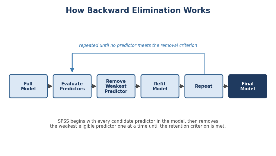
For linear regression specifically, IBM SPSS Statistics documentation explains that stepping criteria can be based on either the probability of the F value or the F value itself. Using probability of F, a variable is entered into the model if the significance level of its F value is less than the entry value, and it is removed if the significance level is greater than the removal value. In backward elimination, every predictor starts in the model, and at each step SPSS evaluates whether any predictor’s removal significance exceeds the removal threshold. If so, the weakest one is dropped and the model is refitted.

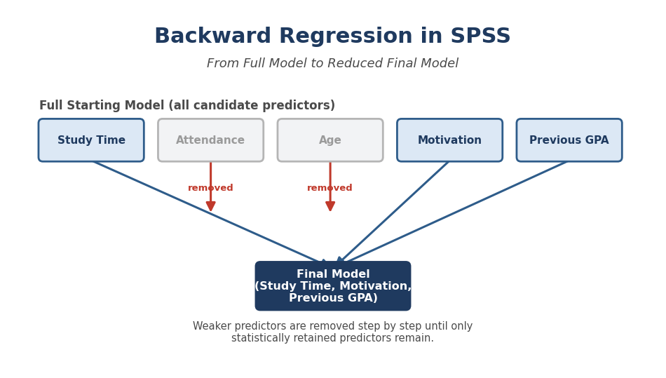
Example: A researcher initially predicts student academic performance from five candidate variables: study time, attendance, age, motivation, and previous academic performance. Backward elimination begins with all five predictors in the model and progressively removes the ones that contribute the least unique explanatory power, potentially leaving a final model with only two or three predictors that meet the retention criterion.

How Backward Elimination Works

Backward elimination follows a consistent logical sequence, regardless of the specific dataset:

1. Enter all candidate predictors. Every variable the researcher wants considered is placed in the independent variables list.
2. Estimate the full regression model. SPSS calculates coefficients, standard errors, and significance values for all predictors simultaneously.
3. Identify the predictor that meets the removal criterion. This is typically the predictor with the highest p-value above the removal threshold (the default removal probability in SPSS linear regression is .10).
4. Remove that predictor. The weakest contributing variable is dropped from the model.
5. Re-estimate the model. SPSS recalculates the regression with the remaining predictors.
6. Repeat the process. Steps 3 through 5 continue for as many steps as needed.
7. Stop when no remaining predictor satisfies the removal criterion. The final step becomes the reported final model.

Because the entry and removal criteria are configurable, it is worth checking the exact values used in a given analysis rather than assuming SPSS’s defaults were applied. IBM SPSS documentation remains the authoritative reference for version specific default values and dialog options, since minor interface details can change between releases.

Backward Regression vs Standard Multiple Regression

The Enter method and the Backward method both start from the same list of predictors, but they diverge sharply after that.

Feature	Enter Method	Backward Method
Starting predictors	All predictors	All predictors
Predictor removal	None automatically	Sequential
Researcher control	High	Partly algorithmic
Primary purpose	Theory testing or model estimation	Variable selection
Best suited for	Confirmatory models	Exploratory or model selection situations
Main limitation	May retain weak predictors	Selection instability and biased inference

The practical implication is that Enter regression is generally the better choice when a researcher has a specific, theory driven hypothesis about which predictors belong in the model, the kind of confirmatory analysis common in hypothesis testing dissertation chapters. Backward regression, by contrast, is better suited to exploratory situations where the goal is to reduce a long candidate list down to the predictors that show the strongest statistical contribution, with the understanding that the resulting model reflects the sample at hand and may not replicate perfectly elsewhere.

Backward vs Forward vs Stepwise Regression in SPSS

These four SPSS regression methods are often confused, but they behave differently at every stage of model building.

Feature	Enter	Backward	Forward	Stepwise
Starting model	All predictors	All predictors	No predictors	No predictors
How variables enter	All at once	Not applicable, already in	One at a time, strongest first	One at a time, strongest first
How variables leave	Not applicable	Sequentially, weakest first	Not applicable	Re-evaluated and can be removed at each step
Primary advantage	Full researcher control	Considers full predictor set before reducing	Simple, builds up gradually	Combines entry and removal checks
Main limitation	May include weak predictors	Selection instability	May miss suppressor effects	Most prone to overfitting and instability
Typical application	Confirmatory hypothesis testing	Reducing a large candidate set	Building a small model incrementally	Exploratory model search

These procedures should not be treated as interchangeable, even though they can sometimes produce a similar final model. Because forward and stepwise methods never see the full predictor set simultaneously in the way backward elimination does, they can miss predictors whose importance only becomes apparent when other variables are controlled for, a pattern statisticians call a suppressor effect.

When Should You Use Backward Regression?

Backward regression tends to work well in situations such as:

• Exploratory predictive modeling, where the goal is prediction rather than theory confirmation.
• Reducing a large candidate set of predictors down to a smaller, more manageable set for further analysis.
• Identifying potentially useful predictors in early stage or pilot research.
• Comparing candidate models built from the same starting predictor pool.
• Situations where all predictors can initially be estimated together without severe multicollinearity or small sample estimation problems.

Backward selection is generally less appropriate when a study is built around a small number of theoretically specified predictors, when the sample size is too small to reliably estimate the full starting model, or when the research questions require testing specific, pre-registered hypotheses. Researchers should not automatically remove theoretically important variables simply because an automated procedure produces a particular p-value. A predictor with strong conceptual justification may still deserve reporting or retention even if it does not survive a mechanical removal criterion.

Assumptions of Backward Linear Regression in SPSS

Backward regression relies on the same core assumptions as any multiple linear regression, since it is still ordinary least squares regression underneath the variable selection layer.

Assumption	Meaning	How to Check in SPSS
Continuous dependent variable	The outcome should be measured on an interval or ratio scale	Confirm variable type in Variable View
Appropriate predictor measurement	Predictors should be continuous or properly coded categorical (dummy) variables	Review coding scheme before analysis
Linearity	The relationship between predictors and the outcome should be approximately linear	Scatterplots and partial regression plots
Independence of observations and errors	Residuals should not be correlated across cases	Durbin-Watson statistic where appropriate
Homoscedasticity	Residual variance should be roughly constant across predicted values	Scatterplot of standardized residuals against predicted values
Approximately normally distributed residuals	Residuals should be roughly normal, particularly for small sample inference	Histogram of residuals and Normal P-P plot
Absence of problematic multicollinearity	Predictors should not be too highly correlated with each other	Tolerance and VIF statistics
No excessively influential observations	No single case should disproportionately affect the model	Cook’s distance, standardized residuals, and leverage values

It is worth emphasizing that multiple linear regression does not require every individual predictor variable to be normally distributed. The normality assumption applies to the residuals of the fitted model, not to the raw distribution of each independent variable.

How to Perform Backward Regression in SPSS

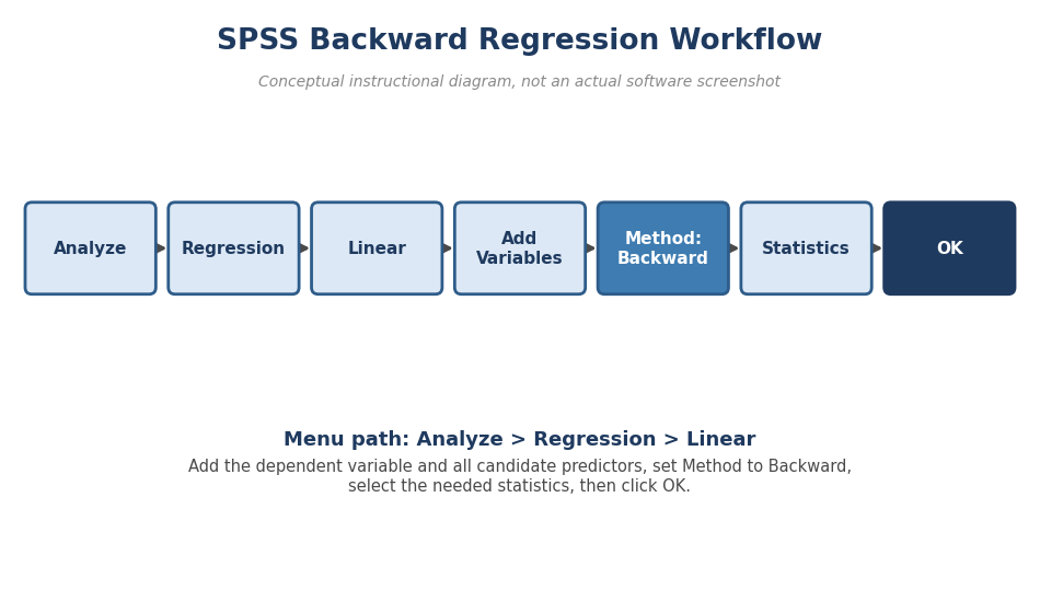
Menu path: Analyze > Regression > Linear

Step 1: Open the Linear Regression Dialog

From the SPSS menu bar, select Analyze, then Regression, then Linear. This opens the main Linear Regression dialog box where the dependent variable, predictors, and method are specified.

Step 2: Select the Dependent Variable

Move the outcome variable into the Dependent box. This variable should normally be continuous (interval or ratio scaled), such as a test score, income figure, or performance index.

Step 3: Add the Independent Variables

Move every candidate predictor into the Independent(s) box. Unlike a confirmatory Enter model, backward elimination requires that all variables under consideration be entered at this stage, since the procedure needs the complete starting model before it can begin removing predictors.

Step 4: Select the Backward Method

Click the Method dropdown menu, which defaults to Enter, and change it to Backward. This tells SPSS to estimate the full model first and then apply the removal criterion at each subsequent step.

Step 5: Select Statistics

Click the Statistics button and choose options that support proper interpretation:

• Estimates produce the unstandardized and standardized coefficients for each step.
• Model fit reports R, R squared, adjusted R squared, and the ANOVA table for each model.
• R squared change shows how much explanatory power is gained or lost at each step, useful for understanding the effect of each removed predictor.
• Confidence intervals provide a range of plausible values for each coefficient, which strengthens APA style reporting.
• Descriptives summarize means, standard deviations, and correlations among variables.
• Part and partial correlations help clarify each predictor’s unique contribution relative to the others.
• Collinearity diagnostics produce tolerance and VIF values needed to check for multicollinearity.

Step 6: Check Regression Diagnostics

Under Plots, request a scatterplot of ZRESID against ZPRED to check homoscedasticity, along with a Normal P-P plot of the regression residuals. Under Save, consider saving standardized residuals and Cook’s distance values to identify influential cases.

Step 7: Run the Analysis

Click OK. SPSS estimates the full model, applies the backward removal criterion at each step, and produces a separate set of output tables for every step in the elimination sequence, concluding with the final retained model.

Quick reference summary:

1. Click Analyze.
2. Select Regression.
3. Select Linear.
4. Add the dependent variable.
5. Add all candidate predictors.
6. Choose Backward under Method.
7. Select relevant statistics and diagnostics.
8. Click OK.

SPSS Syntax for Backward Regression

For researchers who prefer syntax over the dialog boxes, the equivalent command uses the /METHOD=BACKWARD keyword. In this hypothetical example, performance is the dependent variable and study_time, attendance, motivation, and previous_grade are the candidate predictors.

REGRESSION
  /DESCRIPTIVES MEAN STDDEV CORR
  /STATISTICS COEFF OUTS R ANOVA CI(95) TOL
  /DEPENDENT performance
  /METHOD=BACKWARD study_time attendance motivation previous_grade.

• /DESCRIPTIVES requests means, standard deviations, and a correlation matrix for all variables.
• /STATISTICS requests coefficients, excluded variable statistics, R, the ANOVA table, 95% confidence intervals, and tolerance values.
• /DEPENDENT specifies the outcome variable.
• /METHOD=BACKWARD lists the candidate predictors and instructs SPSS to apply backward elimination.

These variable names are hypothetical examples only, used to illustrate correct syntax structure rather than a real dataset.

How to Interpret Backward Regression Output in SPSS

Variables Entered/Removed

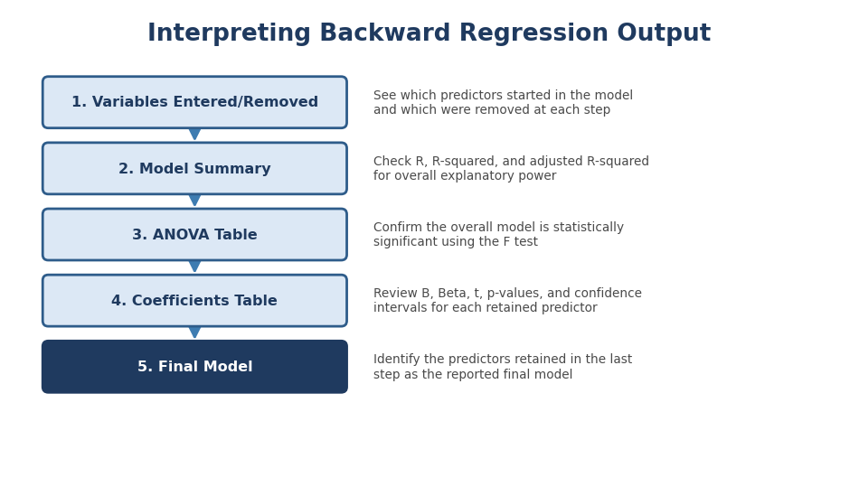
This table lists which predictors started in the model and which single predictor SPSS removed at each numbered step. Reading down the table shows the elimination sequence. The last row before no further removals occur represents the final retained model. The predictors that remain at that final step are the ones the analysis identifies as meeting the retention criterion.

Model Summary

This table reports R (the multiple correlation between the observed and predicted values), R squared (the proportion of variance in the dependent variable explained by the model), adjusted R squared (R squared corrected for the number of predictors and sample size), and the standard error of the estimate (the typical distance between observed and predicted values). When R squared change is requested, it shows how much explained variance was lost when a predictor was removed at each step. Adjusted R squared is particularly useful when comparing models with different numbers of predictors, since raw R squared can only stay the same or increase as predictors are added, while adjusted R squared penalizes the inclusion of predictors that do not meaningfully improve model fit.

ANOVA Table

The ANOVA table reports the F statistic, its associated degrees of freedom, and the significance value for the model at each step. This is a test of the overall model, whether the set of predictors, taken together, explains a significant amount of variance in the outcome. A significant overall F test indicates the model as a whole is useful, but it does not mean that every individual predictor within that model is statistically significant. That determination comes from the coefficients table.

Coefficients Table

For the final model, this table shows:

• Unstandardized B, the predicted change in the outcome for a one unit change in the predictor, holding other predictors constant.
• Standard error, the precision of the B estimate.
• Standardized Beta, the coefficient expressed in standard deviation units, useful for comparing the relative strength of predictors measured on different scales.
• t statistic and p-value, used to test whether each individual predictor’s contribution is statistically significant.
• Confidence interval, the plausible range for the true population coefficient.
• Tolerance and VIF, collinearity diagnostics. Low tolerance (or high VIF) signals that a predictor is highly correlated with other predictors in the model.

The predictors retained in the final model are simply those still listed in the coefficients table at the last step shown in the Variables Entered/Removed table.

Excluded Variables

This table lists predictors that were removed during the elimination process, along with their beta-in value (the standardized coefficient they would have had if re-entered) and significance level at each step. An excluded predictor is not automatically unimportant in every theoretical or substantive sense. It simply did not meet the statistical removal criterion applied to this particular sample, given the other predictors already in the model.

Worked Backward Regression Example

• Research question: Which factors best predict student academic performance?
• Dependent variable: Academic performance score
• Candidate predictors: Study hours, attendance, age, motivation score, previous GPA

Using hypothetical values only, suppose the full starting model includes all five predictors. At Step 1, age shows the highest non-significant removal probability and is dropped first, since it contributes the least unique explanatory power once the other four predictors are accounted for. At Step 2, attendance also fails to meet the retention threshold once age has been removed, and it is dropped next. By Step 3, the remaining three predictors, study hours, motivation score, and previous GPA, all meet the retention criterion, and elimination stops.

In this hypothetical final model, previous GPA and study hours might show positive standardized coefficients, indicating that higher prior performance and more study time are associated with higher predicted academic performance, while motivation score contributes a smaller but still significant positive effect. The adjusted R squared for this hypothetical three predictor model might be similar to or only slightly lower than the five predictor starting model, illustrating that the two removed predictors were not adding meaningful explanatory power once the retained predictors were considered.

This kind of sequence, not the specific numbers, is what a researcher should focus on reporting: which variables were removed, in what order, and what the final retained model implies about the strongest predictors in the sample.

Need help performing or interpreting backward regression in SPSS? Get professional SPSS data analysis support for your dissertation, thesis, or research project.

How to Report Backward Regression Results in APA Style

APA reporting example using hypothetical data

A backward linear regression was conducted to predict academic performance from study hours, attendance, age, motivation score, and previous GPA. Two predictors (age and attendance) were removed across two steps, leaving a final model with three predictors. The final model was statistically significant, F(3, 96) = 24.51, p < .001, R² = .43, adjusted R² = .41. Previous GPA was the strongest predictor (B = 0.52, SE = 0.08, β = .48, t = 6.50, p < .001, 95% CI [0.36, 0.68]), followed by study hours (B = 0.31, SE = 0.09, β = .27, t = 3.44, p = .001, 95% CI [0.13, 0.49]) and motivation score (B = 0.18, SE = 0.07, β = .19, t = 2.57, p = .012, 95% CI [0.04, 0.32]).

Reusable reporting template

A backward linear regression was conducted to predict [outcome] from [list of candidate predictors]. [Number] predictor(s) were removed across [number] step(s), leaving a final model with [number] predictors. The final model was statistically significant, F(df1, df2) = XX.XX, p = XXX, R² = XX, adjusted R² = XX. [Predictor] was the strongest predictor (B = X.XX, SE = X.XX, β = .XX, t = X.XX, p = XXX, 95% CI [X.XX, X.XX]), followed by [additional predictors with the same statistics].

Limitations of Backward Regression

Backward regression is a useful exploratory tool, but it carries well documented statistical risks that dissertation researchers need to understand and disclose.

• Data-driven variable selection. The final model reflects patterns in this specific sample, not necessarily the underlying population relationship.
• Model instability. A slightly different sample could produce a different sequence of removals and a different final model.
• Sample dependence. Results may not replicate well in an independent dataset.
• Inflated Type I error risk. Testing many predictors for removal across multiple steps increases the chance of false positive retention.
• Biased coefficients and standard errors. Coefficients and p-values reported for a model selected through the same data used to test it are generally optimistic and should be interpreted cautiously.
• Overfitting. The selected model may fit the sample better than it fits the broader population.
• Reproducibility difficulty. Backward elimination applied to a new sample from the same population will not always select the same predictors.
• Ignoring theoretical importance. Statistically weak predictors may still be conceptually essential to a study’s framework.
• Multicollinearity effects on selection. Highly correlated predictors can lead to the removal of a theoretically meaningful variable simply because a correlated partner was retained instead.
• No substitute for subject matter expertise. Automated procedures identify statistical patterns, not causal or theoretical importance.

Where possible, researchers should favor theory driven model specification for confirmatory hypotheses, use a validation or holdout sample to check whether the selected model generalizes, consider cross validation techniques, run sensitivity analyses with alternative predictor sets, and always report the variable selection procedure transparently, including the specific entry and removal criteria used.

Backward Linear Regression vs Backward Logistic Regression in SPSS

These are not the same analysis, and they should not be treated interchangeably.

Linear regression is normally used when the dependent variable is continuous, such as a test score or income level. Binary logistic regression is used instead when the outcome variable contains exactly two categories, such as pass or fail. SPSS’s logistic regression procedure offers its own family of backward methods, Backward Conditional, Backward Likelihood Ratio (LR), and Backward Wald, which use different underlying test statistics than the probability-of-F criterion used in linear regression. IBM SPSS documentation on the Regression module describes these as separate stepwise options specific to logistic regression, each with its own entry and removal test (likelihood-ratio, Wald, or conditional statistics) and its own interpretation requirements. A researcher working with a categorical outcome variable should consult the logistic regression procedure specifically rather than applying the linear regression backward workflow described in this guide.

Common Mistakes When Using Backward Regression in SPSS

1. Choosing Backward simply because it produces fewer predictors. Correction: select a method based on the research question and theoretical framework, not on how many predictors survive.
2. Ignoring regression assumptions. Correction: check linearity, homoscedasticity, residual normality, and multicollinearity before trusting the output.
3. Removing theoretically important confounders automatically. Correction: consider forcing key theoretical variables into the model rather than allowing automatic removal.
4. Interpreting p-values without examining effect sizes. Correction: report standardized betas and confidence intervals alongside significance values.
5. Ignoring multicollinearity. Correction: review tolerance and VIF values before finalizing interpretation.
6. Reporting only the final model without describing the selection procedure. Correction: report the starting predictor list, the removal criterion, and the number of steps.
7. Confusing backward linear regression with backward logistic regression. Correction: match the regression procedure to the measurement level of the dependent variable.
8. Treating the selected model as guaranteed to replicate. Correction: describe the model as sample specific and consider validation in an independent dataset.
9. Failing to validate the model. Correction: where feasible, apply cross validation or a holdout sample to check model stability.

Backward Regression for Dissertation Research

Before applying backward regression to a dissertation dataset, it is worth pausing to check whether the method actually fits the study’s design. Researchers should consider whether backward elimination is consistent with their specific research questions, whether it aligns with the hypotheses stated in earlier chapters, whether it fits the conceptual or theoretical framework guiding the study, whether the dissertation methodology chapter already commits to a particular modeling approach, whether a supervisor or committee expects a confirmatory rather than exploratory analysis, and whether the dataset actually satisfies the assumptions required for valid regression inference.

Choosing a regression method solely because it produces statistically significant results is not a defensible methodological justification, and committee members reviewing a results chapter will often ask directly why a particular variable selection method was chosen. A brief, well reasoned justification tied to the research question, rather than the output, strengthens both the analysis and its defense.

Do You Need Help With Backward Regression in SPSS?

Backward regression involves more than a single menu selection. It requires choosing the right method for the research design, testing assumptions correctly, and interpreting a sequence of output tables accurately. spssdissertationhelp.com supports researchers with:

• Choosing an appropriate regression model for their research questions
• Preparing and cleaning datasets for analysis
• Testing regression assumptions
• Running SPSS analyses, including backward, forward, stepwise, and hierarchical regression
• Interpreting SPSS output in plain language
• Producing publication-ready tables and figures
• Writing results sections
• APA 7 statistical reporting
• Responding to supervisor or committee statistical corrections

Need help performing or interpreting backward regression in SPSS? Get professional SPSS data analysis support for your dissertation, thesis, or research project.

Get SPSS Analysis Help

Frequently Asked Questions About Backward Regression in SPSS

Conclusion

Backward regression in SPSS offers a structured way to reduce a large set of candidate predictors down to those that contribute the most statistical explanatory power, starting from the full model and removing the weakest predictors step by step. Running it correctly means entering all candidate predictors, selecting Backward under Method, requesting the right statistics and diagnostics, and reading the output tables in sequence, from Variables Entered/Removed through to the final Coefficients table. Interpreting the final model correctly also means recognizing what the procedure cannot tell you: statistical significance in this sample does not guarantee replication in another, and removed variables are not automatically unimportant in a theoretical sense. Assumption checks, multicollinearity diagnostics, and a clear rationale tied to the research question all remain essential, regardless of which variable selection method is chosen.

Need expert help with backward regression in SPSS? Whether the task is choosing between regression methods, testing assumptions, running the analysis, interpreting output, or writing an APA 7 results section, professional support can help dissertation and thesis researchers move through this stage with confidence.

Get SPSS Analysis Help