Difference Between Pearson and Spearman Correlation: Foundations, Theory, and Research Context

Understanding the difference between Pearson and Spearman correlation is one of the most important foundational skills in quantitative research. Although correlation analysis appears straightforward at first glance, selecting the wrong correlation coefficient can compromise the validity of results, weaken dissertation defenses, and trigger major revisions during peer review. Many students assume both statistics measure the same concept and differ only slightly in calculation. In reality, they rest on different statistical assumptions, theoretical foundations, and interpretative frameworks.

Correlation analysis is not simply about generating a number between minus one and plus one. It is about understanding how variables behave, how data are distributed, and how relationships unfold across values. When researchers choose Pearson correlation, they are making a parametric assumption about linear association. When they choose Spearman correlation, they are selecting a nonparametric approach designed to evaluate monotonic patterns without requiring strict distributional assumptions.

Before diving into mathematical differences, it is essential to understand what correlation actually represents in scientific inquiry.

What Correlation Means in Quantitative Research

Correlation measures the degree to which two variables move together. It does not test causation. It does not prove influence. It does not establish directionality. Instead, it quantifies association. In practical research terms, correlation helps answer questions such as:

• Does increased study time relate to improved academic performance?
• Is job satisfaction associated with employee retention?
• Does advertising expenditure relate to revenue growth?
• Is body mass index associated with blood pressure levels?

In each of these scenarios, correlation provides insight into whether variables tend to increase together, decrease together, or show no systematic pattern. A correlation coefficient ranges from -1 to +1. The magnitude reflects strength, and the sign reflects direction.

• A value close to +1 indicates a strong positive association.
• A value close to -1 indicates a strong negative association.
• A value near zero indicates little or no association.

However, the way this coefficient is calculated differs significantly between Pearson and Spearman.

The Statistical Philosophy Behind Pearson Correlation

Pearson correlation, formally known as the Pearson Product-Moment Correlation Coefficient, measures the strength and direction of a linear relationship between two continuous variables. The word “linear” is critical. Pearson assumes that the relationship between variables can be described using a straight line. If one were to plot data points on a scatterplot and visually observe a pattern that resembles a straight upward or downward slope, Pearson correlation becomes appropriate. The statistic essentially measures how closely data points cluster around an imaginary best-fit line. Mathematically, Pearson correlation is calculated based on the covariance between variables divided by the product of their standard deviations. Because it relies directly on raw numerical values, it is highly sensitive to extreme observations and distributional shape.

The theoretical assumptions underlying Pearson correlation include:

• Both variables are measured at the interval or ratio level.
• The relationship is linear.
• Data are approximately normally distributed.
• Homoscedasticity exists, meaning variance remains consistent across levels.
• Outliers are minimal or absent.

These assumptions make Pearson a parametric statistic. Parametric methods rely on specific distributional expectations. When these assumptions hold true, Pearson is powerful and efficient. When they are violated, results may be distorted.

The Statistical Philosophy Behind Spearman Correlation

Spearman correlation, also known as Spearman’s Rank-Order Correlation Coefficient, approaches association differently. Rather than analyzing raw values directly, Spearman converts data into ranks before computing the correlation. This transformation makes Spearman a nonparametric statistic. Nonparametric tests do not require normal distribution assumptions and are less affected by extreme values. Spearman measures monotonic relationships. A monotonic relationship means that as one variable increases, the other tends to increase or decrease consistently, though not necessarily in a straight-line fashion. For example, imagine income and happiness. Happiness may increase rapidly with income at lower levels but plateau at higher income levels. This relationship may not be linear, but it may still be monotonic. Spearman can detect that consistent directional pattern.

Spearman correlation is particularly useful when:

• Data are ordinal (such as Likert-scale responses).
• Normality assumptions are violated.
• Outliers distort parametric measures.
• The scatterplot shows a curved but consistent pattern.

Because it relies on ranks, Spearman reduces the influence of extreme observations and skewed distributions.

Linear Versus Monotonic Relationships

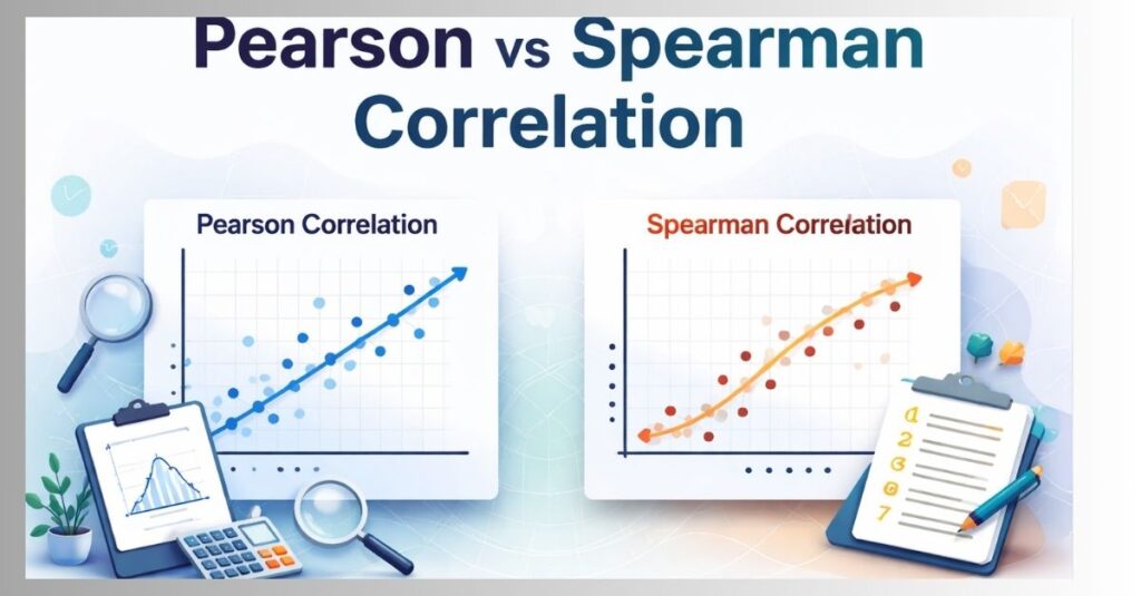
The distinction between linear and monotonic relationships represents the most important conceptual difference between Pearson and Spearman correlation. A linear relationship implies proportional change. If X increases by a certain amount, Y increases or decreases at a constant rate. The points on a scatterplot align along a straight line. A monotonic relationship implies consistent direction but not constant rate. Y may increase rapidly at first and then slow down, or it may decrease gradually and then sharply. As long as the direction remains consistent, the relationship is monotonic. All linear relationships are monotonic, but not all monotonic relationships are linear.

• Pearson measures only linear relationships.
• Spearman measures monotonic relationships, including linear ones.

This distinction is critical in dissertation research. Many students incorrectly apply Pearson when data exhibit nonlinear but monotonic trends. This can underestimate association strength and lead to misleading interpretations.

Measurement Scales and Their Role in Correlation Selection

Measurement level determines statistical eligibility.

Interval and ratio data support parametric testing. Examples include:

• Income
• Temperature
• Age
• Test scores
• Weight
• Reaction time

Ordinal data represent ranked categories without equal intervals between points. Examples include:

• Satisfaction ratings (1–5 scale)
• Agreement levels
• Performance rankings
• Socioeconomic class categories

Pearson requires interval or ratio data.
Spearman works with ordinal, interval, or ratio data.

In survey-based dissertation research, especially when using Likert scales, many researchers choose Spearman to remain conservative. Others justify treating Likert scales as interval data and use Pearson. The decision must align with field norms and supervisor guidance. For more on preparing ordinal survey datasets correctly, see Survey Data Analysis.

Sensitivity to Outliers

Outliers represent another critical difference.

Pearson correlation uses raw values. A single extreme data point can dramatically inflate or deflate the coefficient. This is because covariance calculations depend on distance from the mean.

Spearman correlation uses ranks. Even if one value is extremely large, its rank position may not distort the overall pattern significantly. Therefore, Spearman is considered more robust to outliers.

In applied research contexts such as healthcare, finance, and psychology, outliers frequently appear. Choosing the wrong method may compromise findings.

Before running correlation, researchers should perform:

• Boxplot inspection
• Z-score outlier checks
• Mahalanobis distance testing when appropriate

Normality Assumptions

Normal distribution plays a key role in parametric statistics.

Pearson correlation assumes both variables are approximately normally distributed. This assumption is especially important when sample sizes are small.

Spearman correlation does not require normal distribution.

In large samples, normality violations may have minimal effect due to the Central Limit Theorem. However, dissertation committees often require formal testing using:

• Shapiro-Wilk test
• Kolmogorov-Smirnov test
• Q-Q plots
• Histograms

Failure to check assumptions frequently leads to examiner comments requesting reanalysis.

Strength of Association Interpretation

Although Pearson and Spearman coefficients share the same numeric range, interpretation must consider context.

General guidelines suggest:

• 0.10 indicates small association
• 0.30 indicates moderate association
• 0.50 or above indicates strong association

However, these thresholds vary by discipline. In behavioral sciences, correlations above 0.40 are often meaningful. In physical sciences, higher thresholds may be expected.

Researchers should always report:

• Correlation coefficient
• Significance level
• Sample size
• Confidence intervals if available

For assistance in structuring academic results sections, review Dissertation Results Help.

Practical Research Scenario Comparison

Imagine a researcher examining the relationship between:

• Variable A: Hours of sleep
• Variable B: Cognitive performance score

If both variables are continuous and normally distributed with a straight-line relationship, Pearson is appropriate.

Now imagine:

• Variable A: Satisfaction rating (1–5)
• Variable B: Loyalty ranking

Because at least one variable is ordinal, Spearman is likely more appropriate.

These decisions are not cosmetic. They affect methodological defensibility.

Why Choosing the Correct Correlation Matters

Examiners and peer reviewers often focus heavily on methodological decisions. Incorrect statistical choice signals weak understanding of research design. Many dissertation revisions involve comments such as:

• Justify choice of correlation coefficient.
• Test assumptions before applying Pearson.
• Explain why Spearman was selected instead of Pearson.
• Clarify measurement level of variables.

Making the correct choice from the beginning reduces revision cycles and strengthens academic credibility.

If you are unsure about method selection, you may request professional dataset review through SPSS Correlation Analysis Help.

Transition to Deeper Technical Comparison

Now that we have covered foundational theory, measurement scales, assumptions, and conceptual differences, the next section will explore:

• Mathematical differences in calculation
• Detailed assumption diagnostics
• Advanced research scenarios
• Interpretation nuances
• Effect size considerations
• Field-specific application guidance

Mathematical Foundations, Assumption Testing, Statistical Power, and Technical Distinctions

A deeper understanding of Pearson and Spearman correlation requires moving beyond conceptual definitions into the mechanics of how each statistic is calculated and why their assumptions matter. Many dissertation errors occur not because students misunderstand what correlation measures, but because they do not fully appreciate how the underlying formulas respond to data structure, distribution, and outliers. A strong methodological justification depends on understanding these technical differences.

Both Pearson and Spearman produce coefficients ranging from -1 to +1. However, they reach those values through fundamentally different computational pathways. These differences explain why assumption violations affect one coefficient more than the other and why the same dataset can produce noticeably different results depending on which method is used.

The Mathematical Logic of Pearson Correlation

Pearson correlation is built upon the concept of covariance. Covariance measures the degree to which two variables vary together around their respective means. If values of one variable tend to be above their mean when values of the other variable are also above their mean, covariance will be positive. If one variable is above its mean while the other tends to be below its mean, covariance becomes negative.

However, covariance alone is scale-dependent. Larger measurement units produce larger covariance values. Pearson resolves this by standardizing covariance using the product of both variables’ standard deviations. This standardization ensures that the coefficient always falls between -1 and +1, making interpretation consistent across datasets.

Because Pearson relies on means and standard deviations, it assumes that:

• Data are approximately normally distributed
• Variability is consistent across levels
• The relationship between variables is linear

The dependence on raw values means that each observation influences the final coefficient proportionally to its distance from the mean. Extreme observations, therefore, can exert substantial influence. This is why Pearson is described as sensitive to outliers.

When assumptions are satisfied, Pearson is statistically efficient and powerful. It provides precise estimation of linear relationships and maximizes statistical power under parametric conditions. However, when the relationship is nonlinear or when distributional assumptions are violated, Pearson may underestimate or misrepresent association strength.

The Mathematical Logic of Spearman Correlation

Spearman correlation follows a different computational philosophy. Instead of analyzing raw values directly, it first converts each variable into ranked positions. The smallest value receives rank one, the next smallest rank two, and so on. After this ranking transformation, Pearson correlation is computed on the ranked variables.

This ranking process changes the statistical landscape entirely. The magnitude of differences between values no longer matters. Only relative position matters.

For example, if income values range from 20,000 to 2,000,000, the extreme gap between observations does not inflate the coefficient once ranks are assigned. The highest income receives the highest rank, but the distance between that value and the next highest is irrelevant in the correlation calculation.

This transformation explains why Spearman is less sensitive to outliers and does not require normal distribution. It focuses on order consistency rather than proportional linear change.

Spearman correlation is therefore ideal when:

• Data are ordinal
• Distributions are skewed
• Outliers are present
• The relationship is monotonic but not strictly linear

The ranking step reduces distortion and increases robustness when parametric assumptions cannot be confidently met.

Assumption Testing and Diagnostic Procedures

Before selecting a correlation coefficient, researchers must evaluate data characteristics carefully. Assumption testing is not optional in high-level academic research. It directly informs methodological choice and ensures defensible analysis.

Evaluating Linearity

Linearity is assessed primarily through scatterplots. A linear pattern appears as a straight diagonal clustering of points. If data points curve upward or downward consistently but not in a straight line, the relationship may be monotonic rather than linear.

Failure to inspect scatterplots is one of the most common research errors. A numerical coefficient alone cannot reveal whether the relationship satisfies linear assumptions.

Evaluating Normality

Normality testing involves examining whether the distribution of each variable approximates a bell-shaped curve.

Researchers commonly use:

• Shapiro-Wilk test
• Kolmogorov-Smirnov test
• Histograms
• Q-Q plots
• Skewness and kurtosis values

Minor deviations from normality may not severely affect Pearson in large samples. However, substantial skewness can distort covariance and reduce interpretive reliability.

When normality is violated, Spearman provides a nonparametric alternative that does not rely on distributional symmetry.

Homoscedasticity and Variance Consistency

Homoscedasticity refers to equal variance across levels of one variable relative to another. In correlation analysis, it implies that the spread of points around the best-fit line remains consistent.

If scatterplots show widening or narrowing dispersion patterns, heteroscedasticity may be present. Pearson assumes variance consistency. Severe violations can weaken interpretability and reduce model reliability.

Spearman correlation does not depend on variance structure in the same parametric sense because it operates on ranked data rather than modeling proportional deviation from means.

Handling Tied Ranks in Spearman Analysis

In applied research, particularly in survey-based studies, tied values frequently occur. For example, many respondents may select the same Likert response option. When ties occur, statistical software assigns average ranks to tied values.

While tied ranks slightly reduce the maximum possible coefficient magnitude, they do not invalidate Spearman analysis. Modern statistical software adjusts calculations automatically to maintain accuracy.

When working with ordinal survey responses, consider reviewing Survey Data Analysis to ensure proper dataset preparation before correlation testing.

Statistical Power and Efficiency

When all parametric assumptions are satisfied, Pearson correlation generally has greater statistical power than Spearman. Statistical power refers to the probability of correctly detecting a true relationship.

However, this advantage disappears when assumptions are violated. If nonlinearity, skewness, or extreme outliers are present, Pearson may produce misleading coefficients or inflated Type I and Type II error rates.

Spearman may sacrifice slight efficiency under ideal parametric conditions but gains robustness when assumptions are uncertain.

Therefore, the choice between Pearson and Spearman involves balancing statistical power with assumption validity.

Sample Size Considerations

Sample size influences both coefficients.

With small samples:

• Pearson estimates may become unstable if distributional assumptions are not satisfied.
• Spearman often provides more reliable estimates due to its nonparametric nature.

With large samples:

• Minor normality violations become less problematic.
• Statistical significance becomes easier to achieve, even for weak associations.

Researchers should interpret correlation magnitude alongside sample size rather than relying solely on p-values.

Sensitivity to Nonlinear but Monotonic Patterns

Consider a dataset in which productivity increases rapidly with training hours at first and then levels off. The relationship is upward but curved.

Pearson may underestimate the strength because it attempts to fit a straight line to a curved pattern. Spearman, however, captures consistent directional ranking and may report a stronger coefficient.

This difference demonstrates why scatterplot inspection is essential before selecting a method.

Partial Correlation and Advanced Extensions

Pearson correlation extends naturally into partial correlation, which examines the relationship between two variables while controlling for a third variable. This extension is common in social sciences and health research.

Spearman also allows for rank-based partial correlation, though it is less commonly used in basic dissertation research.

When research design involves multiple predictors or confounding variables, correlation often transitions into regression modeling. For guidance on this progression, consult Multiple Regression Analysis in SPSS.

Significance Testing and Hypothesis Framework

Correlation analysis typically tests the null hypothesis that no association exists between variables. Significance values indicate whether the observed coefficient differs statistically from zero.

Two-tailed testing is standard unless strong theoretical justification supports directional hypotheses.

Researchers should integrate statistical significance with effect size interpretation. Large samples may produce statistically significant but practically trivial correlations. Effect size discussion should always align with theoretical context.

For structured reporting support, review Dissertation Results Help.

Practical Consequences of Incorrect Selection

Choosing Pearson when assumptions are violated can lead to:

• Underestimated or inflated coefficients
• Misleading interpretations
• Reviewer or examiner criticism
• Required reanalysis

Choosing Spearman unnecessarily when assumptions are satisfied may slightly reduce statistical power but generally does not compromise validity.

Methodological defensibility depends on documented assumption testing and clear justification.

If you are uncertain about method selection for your dataset, consider requesting professional review through Correlation Analysis in SPSS

Summary of Technical Distinctions

The core technical differences between Pearson and Spearman arise from:

• Raw value versus ranked data computation
• Linear versus monotonic relationship measurement
• Parametric versus nonparametric assumption structure
• Sensitivity versus robustness to outliers
• Dependence versus independence from normal distribution

Understanding these distinctions ensures accurate statistical modeling and strengthens research credibility.

Applied SPSS Implementation, Dissertation Case Studies, Interpretation Pitfalls, and Decision Framework

Moving from theoretical distinctions to practical application is where many researchers encounter difficulty. Understanding the difference between Pearson and Spearman correlation conceptually is important, but correctly implementing and defending that choice in SPSS output, dissertation chapters, and peer-reviewed manuscripts is what ultimately determines academic success. This section focuses on real-world research execution, interpretation depth, practical decision frameworks, and common errors that examiners frequently highlight.

Correlation analysis may appear simple within statistical software. However, interpretation mistakes, incorrect assumption checks, and poor methodological justification can undermine otherwise solid research. A rigorous and structured approach ensures defensible results.

Running Pearson and Spearman Correlation in SPSS: Detailed Workflow

Although SPSS makes correlation analysis straightforward, researchers must proceed carefully and deliberately.

Step 1: Preliminary Data Screening

Before running any correlation, dataset integrity must be verified. Researchers should examine:

• Missing values
• Coding errors
• Outliers
• Distribution shape
• Measurement scale

Descriptive statistics should be generated first. Frequencies, means, and standard deviations provide early insight into anomalies.

Step 2: Visual Inspection Using Scatterplots

Scatterplots provide immediate visual evidence regarding:

• Linearity
• Monotonicity
• Outliers
• Heteroscedasticity

In SPSS:
Graphs → Chart Builder → Scatter/Dot → Simple Scatter

If data points align along a straight diagonal pattern, Pearson is likely appropriate. If the pattern curves but consistently increases or decreases, Spearman may better represent association.

Ignoring scatterplots is one of the most common dissertation-level mistakes.

Step 3: Normality Testing

For Pearson correlation, test normality of both variables.

In SPSS:
Analyze → Descriptive Statistics → Explore → Plots → Normality plots with tests

Interpret:

• Shapiro-Wilk significance (for small samples)
• Skewness and kurtosis values
• Histogram symmetry
• Q-Q plot alignment

If variables significantly deviate from normal distribution, Spearman may be justified.

Step 4: Running the Correlation

In SPSS:
Analyze → Correlate → Bivariate

Select variables and choose:

• Pearson (for linear parametric analysis)
• Spearman (for monotonic nonparametric analysis)

Ensure:

• Two-tailed testing unless hypothesis is directional
• Flag significant correlations
• Request confidence intervals when available

Dissertation Case Study Examples

Case Study 1: Education Research

A doctoral student investigates the relationship between study hours and GPA among university students.

Both variables are continuous, normally distributed, and linear in scatterplot inspection.

Pearson correlation is appropriate.

Result:
r = .48, p < .001

Interpretation:
There is a moderate positive linear association between study hours and GPA.

Case Study 2: Psychology Survey Study

A researcher examines the relationship between perceived stress (measured on a 5-point Likert scale) and sleep quality ranking.

Data are ordinal and slightly skewed.

Spearman correlation is selected.

Result:
ρ = -.39, p = .002

Interpretation:
Higher perceived stress is moderately associated with lower sleep quality in a monotonic pattern.

Case Study 3: Healthcare Research with Outliers

A dataset examines income and hospital visits. Income includes extreme high earners, creating severe skewness.

Pearson correlation yields:
r = .22

Spearman yields:
ρ = .41

After outlier analysis, Spearman provides a more stable estimate of association because ranking reduces extreme value influence.

Interpretation Depth in Academic Writing

Correlation reporting should go beyond numeric output. A strong dissertation results section includes:

1. Statistical statement
2. Effect size interpretation
3. Theoretical implication
4. Comparison with prior research

Example (Pearson):

A statistically significant moderate positive linear relationship was observed between training duration and productivity, r(120) = .46, p < .001. This finding suggests that increased training hours are associated with measurable improvements in employee performance. The strength of association aligns with previous workforce development studies, indicating practical significance within organizational settings.

Example (Spearman):

A significant monotonic association was found between satisfaction ranking and loyalty ranking, ρ = .51, p < .001. As satisfaction increased, loyalty tended to increase consistently, although the relationship did not demonstrate strict linear proportionality.

For structured dissertation reporting assistance, refer to Dissertation Results Help.

Correlation Versus Causation: Clarifying a Critical Misinterpretation

One of the most common academic pitfalls involves interpreting correlation as causation.

Correlation identifies association. It does not prove:

• One variable causes another.
• Direction of influence.
• Mechanism of effect.

Even a correlation of .80 does not establish causality. Experimental or longitudinal designs are required for causal inference.

Examiners often deduct marks when students overstate correlational findings.

Instead of stating:
“Stress causes lower performance.”

Write:
“Higher stress levels were associated with lower performance scores.”

Precision in language reflects statistical maturity.

Decision Framework for Choosing Pearson or Spearman

Researchers can follow this structured decision pathway:

1. Are both variables continuous?
   • If no, consider Spearman.
2. Is the relationship linear?
   • If yes, Pearson may be appropriate.
   • If monotonic but nonlinear, Spearman may be better.
3. Are variables normally distributed?
   • If yes, Pearson is acceptable.
   • If not, consider Spearman.
4. Are extreme outliers present?
   • If yes, examine whether they distort Pearson.
   • Spearman may provide robustness.
5. Does field standard favor one method?
   • Align with discipline norms.

This framework ensures defensible methodological reasoning during dissertation defense.

Advanced Pitfall: Treating Likert Data Incorrectly

Likert-scale data frequently create confusion.

Strictly speaking, Likert responses are ordinal. However, many researchers treat aggregated Likert scales (e.g., summated multi-item scales) as interval data.

When scale reliability is strong and distribution approximates normality, Pearson may be defensible.

When responses are single-item or highly skewed, Spearman may be safer.

Justification must be clearly stated in methodology.

Effect Size Versus Statistical Significance

Large samples can produce statistically significant but trivial correlations.

Example:
r = .08, p < .001

Although statistically significant, the practical effect is weak.

Researchers should discuss magnitude meaningfully, not rely solely on p-values.

Correlation strength interpretation should be contextualized within discipline norms.

Handling Nonlinear But Non-Monotonic Patterns

If scatterplots show U-shaped or inverted-U relationships, neither Pearson nor Spearman may fully capture the pattern.

In such cases, researchers should consider:

• Polynomial regression
• Curve estimation
• Data transformation

Correlation alone may oversimplify complex relationships.

If transitioning into predictive modeling, consult Multiple Regression Analysis in SPSS.

Examiner Feedback Patterns

Common dissertation feedback includes:

• Justify selection of correlation method.
• Provide assumption testing evidence.
• Include scatterplot visualization.
• Clarify measurement level.
• Report confidence intervals.

Proactively addressing these elements reduces revision cycles.

If you would like a professional review before submission, explore Correlation Analysis Help.

Integrating Correlation Within Larger Research Design

Correlation often serves as:

• Preliminary analysis before regression
• Basis for mediation analysis
• Variable screening method
• Exploratory research tool

Correlation results should align logically with research questions and hypotheses.

Strong research design integrates statistical method choice with theoretical framework.

Preparing for Defense Questions

During dissertation defense, examiners may ask:

• Why did you choose Pearson instead of Spearman?
• What assumptions did you test?
• How did you handle outliers?
• Did you inspect scatterplots?
• What would change if assumptions were violated?

Confidence in answering these questions depends on understanding both theoretical and practical differences.

Comprehensive Comparison, Practical Checklist, Extended FAQs, and Research Implementation Strategy

Selecting between Pearson and Spearman correlation is not simply a technical step in SPSS. It is a methodological decision that affects validity, interpretability, examiner feedback, and overall research credibility. By this stage, the theoretical foundations, computational structures, and diagnostic requirements should be clear. This final section synthesizes those insights into a structured comparison, provides a decision checklist for researchers, addresses advanced practical questions, and offers guidance for implementing correlation analysis within dissertations, journal manuscripts, and professional research reports.

Structured Side-by-Side Comparison

The following table consolidates the core distinctions in a practical format for quick reference:

Feature	Pearson Correlation	Spearman Correlation
Type of Statistic	Parametric	Nonparametric
Data Type Required	Continuous (interval/ratio)	Ordinal or continuous
Relationship Measured	Linear	Monotonic
Uses Raw Values	Yes	No (uses ranks)
Sensitive to Outliers	Highly sensitive	More robust
Requires Normality	Yes (ideally)	No
Handles Skewed Data	Poorly	Well
Statistical Power	Higher under ideal conditions	Slightly lower but robust
Common Symbol	r	ρ (rho)

This comparison demonstrates that neither statistic is inherently superior. Each serves a different analytical purpose depending on data structure and research design.

Practical Research Decision Checklist

Before running correlation analysis, researchers should walk through the following structured evaluation:

1. What is the measurement level of each variable?
   • If either variable is ordinal, consider Spearman.
   • If both are continuous, proceed to further diagnostics.
2. Does the scatterplot indicate a linear relationship?
   • If yes, Pearson may be appropriate.
   • If monotonic but curved, Spearman may better represent the relationship.
3. Are both variables approximately normally distributed?
   • If yes, Pearson is defensible.
   • If heavily skewed, Spearman may be safer.
4. Are there extreme outliers?
   • If yes, evaluate whether they distort Pearson results.
   • Spearman reduces outlier influence.
5. What are the standards within the research discipline?
   • Align with field expectations and prior literature.
6. Have assumptions been documented?
   • Always report assumption testing in methodology.

Following this checklist ensures defensible statistical decisions during dissertation defense or peer review.

Integrating Correlation Into Broader Research Design

Correlation rarely stands alone in academic research. It often serves as:

• Preliminary screening before regression analysis
• Foundation for mediation or moderation models
• Exploratory association testing
• Variable selection mechanism

For example, researchers may first examine correlations before conducting regression to ensure meaningful association exists between predictors and outcome variables. If transitioning into predictive modeling, reviewing Multiple Regression Analysis in SPSS can clarify the next analytical step.

Correlation also plays a critical role in validating theoretical frameworks. Strong associations may support hypothesized relationships, while weak associations may suggest reconsideration of conceptual models.

Reporting Correlation in Dissertation Chapters

Correlation results typically appear in Chapter 4 (Results) of a dissertation. Reporting should include:

• Type of correlation used
• Assumption testing summary
• Correlation coefficient
• Significance value
• Sample size
• Interpretation of magnitude
• Theoretical implications

Example (Pearson):

A Pearson correlation analysis revealed a significant moderate positive relationship between employee engagement and productivity, r(210) = .44, p < .001. Assumption testing confirmed linearity and approximate normality. These findings suggest that higher engagement levels are associated with increased productivity outcomes.

Example (Spearman):

A Spearman rank-order correlation demonstrated a significant monotonic association between service satisfaction ranking and customer loyalty ranking, ρ = .52, p < .001. The relationship remained consistent across ranked categories despite slight distributional skewness.

For structured academic formatting support, consult Dissertation Results Help.

Common Advanced Misinterpretations

Even experienced researchers occasionally make interpretation errors. Below are frequent pitfalls:

Mistaking Association for Causation

Correlation identifies co-movement, not cause-and-effect. Causal language should be avoided unless experimental design supports inference.

Ignoring Effect Size

Statistical significance does not equal practical importance. A large sample may produce significant but weak correlations.

Overlooking Nonlinearity

A strong curved pattern may produce a weak Pearson coefficient. Always inspect scatterplots.

Failing to Report Assumption Testing

Examiners frequently request clarification when assumption diagnostics are absent.

Addressing these issues strengthens methodological rigor.

Extended Frequently Asked Questions

What is the core conceptual difference between Pearson and Spearman correlation?

Pearson measures the strength and direction of linear relationships using raw numerical values. Spearman measures the strength and direction of monotonic relationships using ranked data. Pearson assumes normality and linearity, whereas Spearman does not require these parametric assumptions.

Can Spearman be used for continuous data?

Yes. Spearman can be used for continuous data, particularly when assumptions of normality or linearity are violated. However, if data are continuous, normally distributed, and linear, Pearson may provide greater statistical power.

Is Spearman always safer?

Spearman is more robust to outliers and distribution violations, but it is not automatically superior. If Pearson assumptions are fully satisfied, Pearson is more statistically efficient.

Should Likert-scale data use Pearson or Spearman?

This depends on scale structure and discipline norms. Single-item Likert responses are ordinal and often analyzed using Spearman. Multi-item aggregated scales that approximate interval measurement and demonstrate normal distribution may justify Pearson. Clear justification in methodology is essential.

What if Pearson and Spearman give different results?

If coefficients differ substantially, examine scatterplots, distribution shape, and outliers. Differences often indicate nonlinear or skewed relationships. In such cases, Spearman may better represent association.

Does a high correlation guarantee predictive accuracy?

No. Correlation indicates association strength but does not guarantee predictive performance. Predictive modeling requires regression or other inferential frameworks.

How large should a correlation be to matter?

Interpretation depends on field standards and theoretical expectations. A coefficient of .30 may be meaningful in behavioral sciences but weak in engineering contexts. Always contextualize findings within literature.

Methodological Defense Preparation

During dissertation defense, examiners may ask:

• Why did you select this correlation coefficient?
• How did you test assumptions?
• What would change if assumptions were violated?
• How do you interpret the magnitude in practical terms?

Preparation involves:

• Documented assumption testing
• Clear explanation of measurement scales
• Visual inspection evidence
• Literature-supported justification

Researchers who demonstrate understanding of both theoretical and computational differences typically receive fewer methodological challenges.

If you would like a professional review before submission, consider Correlation Analysis Help.

Strategic Implementation for High-Quality Research

To maximize research credibility:

1. Conduct thorough assumption testing.
2. Inspect scatterplots before analysis.
3. Align method choice with theoretical framework.
4. Report effect sizes and confidence intervals.
5. Avoid causal language.
6. Justify methodological decisions clearly.
7. Cross-check interpretation with prior literature.

Following these principles elevates correlation analysis from a routine procedure to a defensible methodological decision.

Final Synthesis

Pearson and Spearman correlation are not interchangeable tools. They are designed for different data conditions and relationship structures.

Pearson is optimal when:

• Variables are continuous
• Distributions approximate normality
• Relationships are linear
• Outliers are minimal

Spearman is optimal when:

• Data are ordinal
• Distributions are skewed
• Outliers are present
• Relationships are monotonic but nonlinear

The decision should always be guided by data characteristics rather than preference.

Selecting the appropriate coefficient strengthens research validity, improves dissertation defense outcomes, and enhances the credibility of published findings.

Request Professional Statistical Review

If you are uncertain about which correlation method best suits your dataset, professional statistical consultation can prevent costly revisions.

Services may include:

• Assumption diagnostics
• Correlation selection guidance
• SPSS output interpretation
• APA-formatted results writing
• Methodology justification drafting

You can request structured support through Request a Quote for Correlation Analysis Support.

Closing Perspective

Mastering the distinction between Pearson and Spearman correlation is not merely about choosing a statistical option in SPSS. It reflects deeper understanding of measurement theory, distributional assumptions, and research design principles.

When selected appropriately and reported rigorously, correlation analysis becomes a powerful tool for advancing theoretical insight and empirical evidence.