
Learning how to run a regression analysis in Stata is important for students, dissertation writers, researchers, and data analysts who need to examine relationships between variables. Regression analysis helps you determine whether one or more independent variables explain or predict changes in a dependent variable.
For example, a student may want to know whether study time predicts exam scores. A business researcher may examine whether service quality predicts customer satisfaction. A healthcare researcher may test whether income, education, and age predict access to healthcare services.
Stata is widely used for quantitative data analysis because it allows researchers to manage datasets, run statistical models, check assumptions, and produce results for academic reporting. However, running regression in Stata is not just about typing one command. You also need to prepare the data, choose the correct variables, understand the output, test assumptions, and explain the findings clearly.
This guide walks you through the full process of running a regression analysis in Stata, from opening your dataset to reporting your results in a dissertation or research paper. If you need support with data cleaning, Stata commands, interpretation, or Chapter 4 writing, SPSS Dissertation Help can assist with the full process.
How Do You Run a Regression Analysis in Stata?
To run a regression analysis in Stata, use the regress command. The dependent variable comes first, followed by the independent variables.
regress dependent_variable independent_variable1 independent_variable2 independent_variable3Example:
regress exam_score study_time attendance ageThis command tells Stata to predict exam_score using study_time, attendance, and age.
| Step | What You Do |
|---|---|
| 1 | Open or import your dataset |
| 2 | Inspect the variables |
| 3 | Check missing values |
| 4 | Confirm variable coding |
| 5 | Identify the dependent variable |
| 6 | Identify the independent variables |
| 7 | Run the regress command |
| 8 | Review the regression output |
| 9 | Check assumptions |
| 10 | Interpret and report the results |
For dissertation work, the most important part is not only running the model. You must also explain whether the model answers your research question, whether the results are statistically significant, and what the findings mean.
What Is Regression Analysis in Stata?
Regression analysis is a statistical technique used to examine the relationship between a dependent variable and one or more independent variables.
The dependent variable is the outcome you want to explain or predict. The independent variables are the predictors that may influence the outcome.
For example:
| Research Question | Dependent Variable | Independent Variable |
|---|---|---|
| Does study time predict exam score? | Exam score | Study time |
| Does service quality predict satisfaction? | Customer satisfaction | Service quality |
| Does income predict savings behavior? | Savings behavior | Income |
| Does leadership style predict engagement? | Employee engagement | Leadership style |
In Stata, the standard command for linear regression is:
regressLinear regression is commonly used when the dependent variable is continuous. Examples of continuous dependent variables include test scores, income, sales revenue, productivity scores, satisfaction ratings, and performance scores.
Regression analysis is useful because it does more than describe your data. It helps you test whether relationships between variables are statistically meaningful. Students who need help choosing the right regression model can also review Regression Analysis Help for more support.
When Should You Use Regression Analysis?
You should use regression analysis when your research question focuses on prediction, explanation, or the relationship between variables.
Regression is useful when you want to answer questions such as:
Does one variable predict another variable?
Does a predictor remain significant after controlling for other variables?
How much does the dependent variable change when an independent variable increases?
Which predictors explain the most variation in the outcome?
Does the evidence support the research hypothesis?
Common dissertation questions that use regression include:
| Dissertation Question | Possible Analysis |
|---|---|
| Does employee training predict job performance? | Linear regression |
| Does service quality predict customer satisfaction? | Linear regression |
| Does financial literacy predict savings behavior? | Linear regression |
| Do income and education predict healthcare access? | Multiple regression |
| Does leadership style predict employee engagement? | Linear regression |
Linear regression is appropriate when your dependent variable is continuous. If your dependent variable is binary, such as yes/no or pass/fail, logistic regression may be more appropriate. If your data follows people, firms, schools, or countries over time, panel regression may be needed.
This page focuses on linear regression using Stata’s regress command. For broader support with statistical methods and dissertation analysis, visit Dissertation Statistics Help.
Types of Regression Used in Stata
Stata can run many types of regression models. The correct model depends on your research question and the type of dependent variable.
| Regression Type | When to Use It | Example Dependent Variable |
|---|---|---|
| Linear regression | Continuous outcome | Exam score, income, satisfaction score |
| Multiple linear regression | Continuous outcome with several predictors | Job performance score |
| Logistic regression | Binary outcome | Yes/no, pass/fail |
| Ordered logistic regression | Ordered categories | Low, medium, high satisfaction |
| Poisson regression | Count outcome | Number of visits |
| Panel regression | Repeated observations over time | Firm-year performance |
This article focuses on ordinary least squares linear regression. More advanced models should be handled separately so the analysis stays focused and clear.
Before Running Regression in Stata
Before running a regression model, make sure your data and research design are ready. Many students make mistakes because they run the command before checking the dataset.
Before you begin, confirm the following:
| Checkpoint | Why It Matters |
|---|---|
| The research question is clear | The model must answer the right question |
| The dependent variable is correct | Stata treats the first variable after regress as the outcome |
| The independent variables are correct | These are the predictors in the model |
| The variables are coded properly | Incorrect coding can lead to wrong interpretation |
| Missing values are checked | Missing data can reduce the regression sample |
| The dependent variable is continuous | Linear regression requires a continuous outcome |
| Assumptions can be tested | Regression results must be reliable |
This preparation is especially important in dissertation research because supervisors and committees often expect students to justify the statistical method used. If you need help preparing your dataset before running the model, Stata Data Analysis Help can support you with data cleaning, coding, missing values, and variable setup.
How Much Sample Size Do You Need for Regression in Stata?
Sample size matters because regression models become less reliable when there are too few observations for the number of predictors. A very small sample can produce unstable coefficients, wide confidence intervals, and weak statistical power.
There is no single sample size rule that works for every dissertation, but students should think about the number of predictors, missing values, expected effect size, and university requirements.
A simple way to think about it is:
| Issue | Why It Matters |
|---|---|
| Too few cases | Results may be unstable |
| Too many predictors | Model may become overfitted |
| Missing values | Stata may exclude cases from the regression |
| Small effect sizes | Larger samples may be needed |
| Control variables | More controls usually require more observations |
For example, a model with 2 predictors is usually easier to support than a model with 12 predictors. If your sample size is small, avoid adding unnecessary variables. Every predictor should be connected to your research question, theory, or literature review.
Before running the final regression, always compare your original sample size with the number of observations Stata uses in the model. If many cases are dropped because of missing data, your final regression sample may be much smaller than expected.
How to Choose Control Variables for Regression
Control variables are variables included in the regression model to account for other factors that may influence the dependent variable. They help you estimate the relationship between your main independent variable and dependent variable more clearly.
For example, if you are studying whether study time predicts exam score, you may control for attendance, age, or prior academic performance. These variables may also influence exam scores, so including them can make your model stronger.
Good control variables usually come from:
| Source | Example |
|---|---|
| Literature review | Prior studies controlled for age and income |
| Theory | A framework suggests education affects the outcome |
| Research design | Demographic factors may influence the dependent variable |
| Committee feedback | Supervisor requests specific controls |
| Practical reasoning | A variable is clearly related to the outcome |
Do not add control variables randomly. Adding too many controls can make the model harder to interpret and may reduce statistical power. A strong regression model should be focused, justified, and connected to the research question.
Step 1: Open or Import Your Dataset in Stata
The first step is opening your dataset in Stata.
If your dataset is already saved as a Stata file, use:
use "dataset.dta", clearIf your data is in Excel, use:
import excel "dataset.xlsx", firstrow clearThe firstrow option tells Stata that the first row of the Excel file contains variable names. The clear option removes any dataset already loaded in Stata.
After importing the data, save it as a Stata file:
save "dataset_clean.dta", replaceSaving your file makes it easier to continue cleaning and analyzing the dataset later.
Step 2: Inspect Your Dataset
After opening the dataset, inspect the data structure. This helps you understand the variable names, labels, data types, and number of observations.
Use:
describeThis command shows the variables in the dataset, their storage types, display formats, and labels.
Next, use:
summarizeThis gives basic descriptive statistics, including the number of observations, mean, standard deviation, minimum, and maximum.
For more detail, use:
summarize, detailThis provides additional information such as percentiles, skewness, and kurtosis.
You can inspect a specific variable with:
codebook variable_nameFor categorical variables, use:
tabulate variable_nameExample:
tabulate genderThese commands help you identify possible issues before running your regression model.
Step 3: Check for Missing Values
Missing values can affect regression analysis because Stata excludes any observation that has missing data in one or more variables used in the model.
To check missing values, use:
misstable summarizeTo check missing values for specific variables, use:
misstable summarize exam_score study_time attendance ageSuppose your original dataset has 300 observations, but your regression output only uses 245 observations. That means 55 cases were excluded because of missing data in one or more variables.
| Stage | Number of Observations |
|---|---|
| Original dataset | 300 |
| Regression sample | 245 |
| Excluded cases | 55 |
This matters because missing values can reduce statistical power and affect the reliability of your findings.
In a dissertation, you may need to explain how missing data was handled. You should not ignore missing values, especially when the number of excluded cases is large.
Step 4: Check Variable Coding
Before running regression, confirm that your variables are coded correctly. This is especially important for categorical variables.
For example, gender may be coded as:
| Code | Meaning |
|---|---|
| 0 | Male |
| 1 | Female |
Or it may be coded as:
| Code | Meaning |
|---|---|
| 1 | Male |
| 2 | Female |
The interpretation of the regression coefficient depends on the coding. If you do not understand how a variable is coded, you may explain the result incorrectly.
Use:
tabulate genderYou can also use:
codebook genderIf you need to create a dummy variable, you can use:
generate female = .
replace female = 1 if gender == 2
replace female = 0 if gender == 1
This creates a variable where female is coded as 1 and male is coded as 0.
Stata also allows factor variable notation. For categorical variables, you can use i. before the variable name:
regress exam_score study_time attendance i.genderThe i.gender tells Stata to treat gender as a categorical variable.
How to Use Dummy Variables in Stata Regression
Dummy variables are used when you want to include categorical variables in regression. A dummy variable usually has two values: 0 and 1.
For example, if gender is coded as male and female, you may create a dummy variable where:
| Dummy Variable | Meaning |
|---|---|
| 0 | Male |
| 1 | Female |
If the coefficient for the dummy variable is positive, it means the group coded as 1 has a higher predicted value than the reference group, holding other variables constant.
You can create a dummy variable manually:
generate female = .
replace female = 1 if gender == 2
replace female = 0 if gender == 1
Or you can use Stata’s factor variable notation:
regress exam_score study_time attendance i.genderUsing i.gender is often easier because Stata automatically treats gender as a categorical variable and chooses a reference category.
Dummy variables are common in dissertation regression models because many studies include demographic variables such as gender, employment status, education level, marital status, or group membership.
Step 5: Identify the Dependent Variable
The dependent variable is the outcome you want to explain or predict. In Stata, the dependent variable comes immediately after the regress command.
Example:
regress exam_score study_time attendance ageIn this command, exam_score is the dependent variable.
For linear regression, the dependent variable should usually be continuous.
| Dependent Variable | Suitable for Linear Regression? |
|---|---|
| Exam score | Yes |
| Income | Yes |
| Customer satisfaction score | Yes |
| Employee engagement score | Yes |
| Sales revenue | Yes |
| Pass/fail status | No |
| Yes/no response | No |
If your dependent variable is not continuous, a different regression model may be better.
Step 6: Identify the Independent Variables
Independent variables are the predictors used to explain the dependent variable.
For example, suppose your research question is:
Does study time predict exam score after controlling for attendance and age?
Your variables would be:
| Role | Variable |
|---|---|
| Dependent variable | exam_score |
| Main independent variable | study_time |
| Control variable | attendance |
| Control variable | age |
The Stata command would be:
regress exam_score study_time attendance ageIn dissertation research, independent variables should come from your research questions, hypotheses, literature review, and conceptual framework.
Do not add predictors randomly. Each variable should have a clear reason for being included in the model.
Step 7: Run the Regression Command in Stata
Once your data is prepared and your variables are selected, run the regression command.
The basic syntax is:
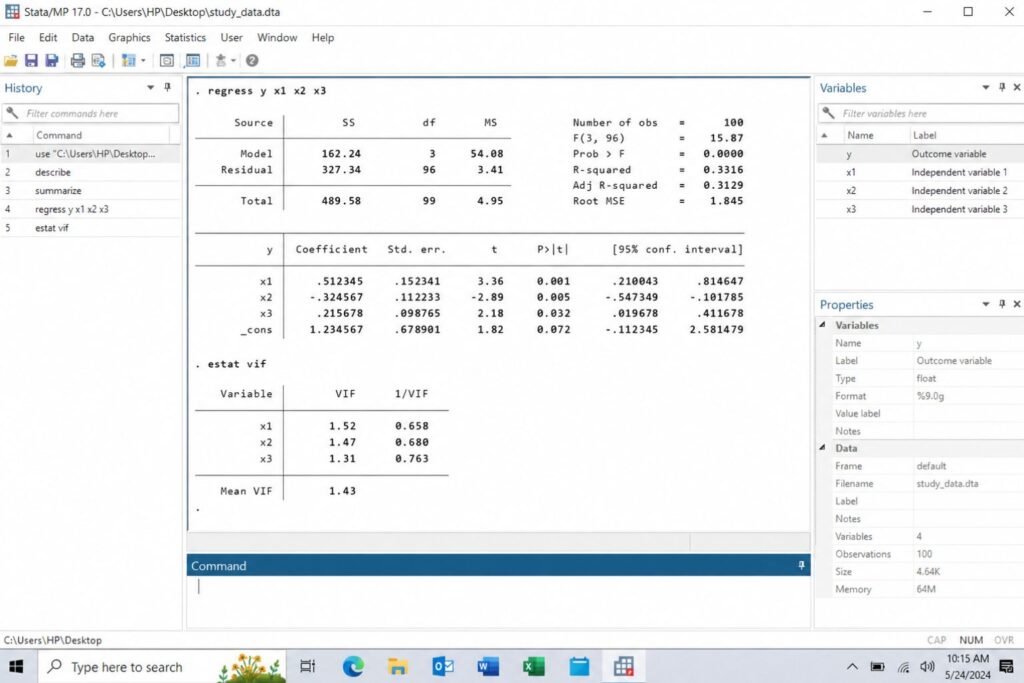
regress y x1 x2 x3Where:
| Symbol | Meaning |
|---|---|
| y | Dependent variable |
| x1 | First independent variable |
| x2 | Second independent variable |
| x3 | Third independent variable |
Example:
regress exam_score study_time attendance ageThis model estimates whether study time, attendance, and age predict exam score.
If you have a categorical predictor, use factor notation:
regress exam_score study_time attendance age i.genderIf you want robust standard errors, use:
regress exam_score study_time attendance age, robustThe regression output will appear in the Stata Results window.
Step 8: Understand the Stata Regression Output
After running the regression command, Stata produces an output table. The output has two main sections.
The top section summarizes the overall model. The lower section shows the results for each independent variable.
The top section usually includes:
| Output Item | Meaning |
|---|---|
| Number of obs | Number of observations used in the model |
| F statistic | Tests whether the overall model is significant |
| Prob > F | P-value for the overall model |
| R-squared | Proportion of variation explained by the model |
| Adjusted R-squared | R-squared adjusted for number of predictors |
| Root MSE | Average prediction error |
The coefficient table usually includes:
| Output Item | Meaning |
|---|---|
| Coef. | Estimated effect of the predictor |
| Std. Err. | Standard error of the coefficient |
| t | Test statistic |
| P> | t |
| 95% Conf. Interval | Lower and upper confidence interval |
For dissertation reporting, the most important values are usually the coefficient, p-value, confidence interval, R-squared, adjusted R-squared, and overall model significance. If you already have output but are unsure what it means, Regression Analysis Help can help you interpret your results correctly.
How to Interpret Regression Coefficients in Stata
The coefficient tells you how much the dependent variable is expected to change when the independent variable increases by one unit, holding other variables constant.
Suppose your regression output looks like this:
| Variable | Coefficient | p-value |
|---|---|---|
| study_time | 2.45 | 0.003 |
| attendance | 0.80 | 0.041 |
| age | -0.12 | 0.511 |
The coefficient for study_time is 2.45. This means each one-unit increase in study time is associated with a 2.45-point increase in exam score, holding attendance and age constant.
The coefficient for attendance is 0.80. This means higher attendance is associated with higher exam scores, holding the other variables constant.
The coefficient for age is negative, but the p-value is 0.511. This means age is not statistically significant in this model.
| Coefficient Direction | Meaning |
|---|---|
| Positive coefficient | As the predictor increases, the outcome increases |
| Negative coefficient | As the predictor increases, the outcome decreases |
| Coefficient close to zero | The predictor has little estimated effect |
| Significant coefficient | The predictor is statistically related to the outcome |
| Non-significant coefficient | There is not enough evidence of a relationship |
The phrase “holding other variables constant” means that the effect of one predictor is estimated while accounting for the other variables in the model.
How to Interpret P-Values in Stata Regression
The p-value helps you determine whether a predictor is statistically significant.
A common rule is:
| P-Value | Interpretation |
|---|---|
| p < .001 | Highly statistically significant |
| p < .01 | Very statistically significant |
| p < .05 | Statistically significant |
| p > .05 | Not statistically significant |
If the p-value for study_time is 0.003, you can say that study time is a statistically significant predictor of exam score.
If the p-value for age is 0.511, you can say that age is not a statistically significant predictor of exam score.
However, p-values should not be interpreted alone. You should also consider the coefficient size, confidence interval, sample size, theory, and practical meaning of the result.
How to Interpret R-Squared in Stata
R-squared shows how much variation in the dependent variable is explained by the independent variables in the model.
For example, if R-squared is 0.42, the model explains 42% of the variation in the dependent variable.
A dissertation-style interpretation could be:
The model explained 42% of the variance in exam score, suggesting that study time, attendance, and age accounted for a meaningful proportion of differences in student performance.
Adjusted R-squared is similar to R-squared, but it adjusts for the number of predictors in the model. It is often useful when comparing models with different numbers of independent variables.
You should not rely only on R-squared. A high R-squared does not automatically mean the model is correct, and a low R-squared does not always mean the model is weak. In many social science, education, business, and healthcare studies, lower R-squared values can still be meaningful.
Step 9: Check Regression Assumptions in Stata
Regression assumptions help determine whether your model is appropriate and whether the results can be trusted.
The main assumptions of linear regression include:
| Assumption | Meaning |
|---|---|
| Linearity | The relationship between predictors and outcome is approximately linear |
| Independence | Observations are independent |
| Normality of residuals | Residuals are approximately normally distributed |
| Homoscedasticity | Residual variance is constant |
| No multicollinearity | Predictors are not too highly correlated |
| No extreme influential outliers | No single case strongly distorts the model |
Check Linearity and Residual Patterns
After running the regression, use:
rvfplotThis creates a residual-versus-fitted plot. Ideally, the residuals should be randomly scattered around zero. Strong patterns may suggest nonlinearity or heteroscedasticity.
Check Normality of Residuals
First, create residuals:
predict residuals, residThen use:
histogram residuals, normalYou can also use:
qnorm residualsThese commands help you check whether residuals are approximately normally distributed.
Check Heteroscedasticity
Use:
estat hettestIf the test is significant, it may suggest heteroscedasticity. In that case, you may consider robust standard errors.
Check Multicollinearity
Use:
vifVIF stands for variance inflation factor. High VIF values may indicate multicollinearity among the independent variables.
A common guideline is that VIF values above 5 or 10 may be a concern, depending on your field and university requirements.
If you need help checking assumptions, interpreting diagnostic tests, or deciding whether robust standard errors are appropriate, Quantitative Data Analysis Help can help you review your model carefully.
Step 10: Run Regression with Robust Standard Errors
If there is evidence of heteroscedasticity, you may run the regression with robust standard errors.
Example:
regress exam_score study_time attendance age, robustThe robust option adjusts the standard errors. This can make p-values and confidence intervals more reliable when the constant variance assumption is violated.
Robust standard errors do not usually change the coefficients. They mainly affect the standard errors, test statistics, p-values, and confidence intervals.
However, robust standard errors do not fix every problem. They do not correct poor model selection, missing variables, incorrect coding, or weak research design.
Step 11: Export Regression Results from Stata
After running regression analysis in Stata, you may need to export the results to Word or Excel for your dissertation.
Common Stata export commands include:
outreg2esttabasdocExample using outreg2:
outreg2 using regression_results.doc, replaceExample using asdoc:
asdoc regress exam_score study_time attendance ageExporting results can help you create clean tables, but the table alone is not enough. You still need to explain the results in your own academic writing.
Step 12: Report Regression Results in a Dissertation
A strong dissertation regression section should explain what analysis was conducted, why it was used, which variables were included, whether the model was significant, and what the findings mean.
You should report:
| Item | What to Include |
|---|---|
| Type of analysis | Linear regression or multiple linear regression |
| Dependent variable | The outcome variable |
| Independent variables | The predictors in the model |
| Model significance | F statistic and p-value |
| Model fit | R-squared and adjusted R-squared |
| Predictor results | Coefficients, standard errors, p-values, confidence intervals |
| Assumption checks | VIF, residuals, heteroscedasticity, outliers |
| Conclusion | Whether the hypothesis was supported |
Example dissertation write-up:
A multiple linear regression was conducted to examine whether study time predicted exam score after controlling for attendance and age. The overall model was statistically significant, F(df1, df2) = X.XX, p < .05, and explained XX% of the variance in exam score. Study time was a statistically significant positive predictor of exam score, b = X.XX, SE = X.XX, p < .05, indicating that higher study time was associated with higher exam scores. Attendance was also a statistically significant predictor, while age was not statistically significant. These findings suggest that study behavior and class attendance are important predictors of student academic performance.
Replace the X values with your actual Stata output.
If you need support writing the results section in a clear academic format, Dissertation Statistics Help can assist with results interpretation, tables, and Chapter 4 reporting.
Full Example: Running Regression Analysis in Stata
Suppose your dissertation topic is:
The effect of study time and attendance on student academic performance.
Your variables are:
| Variable | Role |
|---|---|
| exam_score | Dependent variable |
| study_time | Main independent variable |
| attendance | Independent variable |
| age | Control variable |
| gender | Control variable |
Step 1: Inspect the Data
describe
summarize exam_score study_time attendance age
tabulate gender
misstable summarize
Step 2: Check Correlations
correlate exam_score study_time attendance ageCorrelation helps you see whether variables are related before running the regression. It does not replace regression, but it can provide useful early insight.
Step 3: Run the Regression Model
regress exam_score study_time attendance age i.genderThis command estimates whether study time, attendance, age, and gender predict exam score.
Step 4: Check Multicollinearity
vifThis checks whether the independent variables are too highly related to each other.
Step 5: Check Heteroscedasticity
estat hettestThis tests whether the residual variance is constant.
Step 6: Run Robust Regression if Needed
regress exam_score study_time attendance age i.gender, robustThis runs the same regression model with robust standard errors.
Step 7: Interpret the Findings
If study_time has a positive coefficient and p < .05, you may write:
Study time was a statistically significant positive predictor of exam score. This indicates that students who spent more time studying tended to have higher exam scores, holding attendance, age, and gender constant.
If attendance is significant, you may write:
Attendance was also a statistically significant predictor of exam score, suggesting that students with higher attendance tended to perform better academically.
If age is not significant, you may write:
Age was not a statistically significant predictor of exam score in the model.
Common Mistakes When Running Regression in Stata
Running Regression Before Cleaning the Data
Do not run your final regression before checking your dataset. Missing values, incorrect coding, duplicate cases, and unusual outliers can affect your results.
Using the Wrong Dependent Variable
Linear regression is appropriate for continuous dependent variables. If your outcome is binary, ordinal, categorical, or count-based, another regression model may be more appropriate.
Placing Variables in the Wrong Order
In Stata, the dependent variable comes first.
Incorrect:
regress study_time exam_score ageCorrect:
regress exam_score study_time ageThe incorrect version predicts study time instead of exam score.
Ignoring Missing Values
Stata automatically removes observations with missing values in any variable included in the model. Always compare your original sample size with the number of observations in the regression output.
Misinterpreting P-Values
A p-value tells you whether a result is statistically significant. It does not tell you whether the effect is large, important, or meaningful in practice.
Ignoring Regression Assumptions
Regression assumptions should be checked before final reporting. If assumptions are ignored, your findings may be questioned.
Reporting Output Without Interpretation
A regression table is not enough. You need to explain what each important result means.
Weak reporting:
The coefficient was 2.45 and the p-value was 0.003.
Stronger reporting:
Study time was a statistically significant positive predictor of exam score, b = 2.45, p = .003, indicating that each one-unit increase in study time was associated with a 2.45-point increase in exam score, holding attendance and age constant.
Adding Too Many Variables
Do not add predictors only to increase R-squared. Each variable should be supported by your literature review, research question, or conceptual framework.
Regression Analysis in Stata for Dissertation Research
Regression analysis is one of the most common methods used in dissertation research because it helps test relationships between variables.
Students often use Stata regression analysis in fields such as business, education, economics, healthcare, public health, psychology, political science, nursing, and social science.
Examples include:
| Field | Regression Question |
|---|---|
| Business | Does service quality predict customer satisfaction? |
| Education | Does study time predict academic performance? |
| Healthcare | Do income and education predict healthcare access? |
| Psychology | Does stress predict life satisfaction? |
| Management | Does leadership style predict employee engagement? |
| Finance | Does financial literacy predict savings behavior? |
A strong dissertation regression analysis should include a clear research question, correct model selection, clean data, accurate Stata commands, assumption testing, proper interpretation, and a clear connection to the study’s hypotheses.
For students working on a full research project, SPSS Dissertation Help can support the process from data preparation to results reporting.
Stata Regression Analysis Help for Dissertations
Running a regression command in Stata is only one part of the analysis. Many students can type the regress command, but still struggle with choosing the correct model, preparing the dataset, checking assumptions, interpreting the output, and writing the results clearly in Chapter 4.
At SPSS Dissertation Help, we support students and researchers who need help with Stata regression analysis for dissertations, theses, capstone projects, journal articles, and academic research. Our goal is to help you move from raw data to clear, accurate, and well-explained results.
If you need support preparing your dataset before running the model, our Stata Data Analysis Help service can help with data cleaning, coding, labeling, missing values, and variable setup. If your main challenge is choosing the right model or interpreting coefficients, p-values, confidence intervals, and R-squared, our Regression Analysis Help service can support you through the full regression process.
For students working on thesis or dissertation projects, our Dissertation Statistics Help and Quantitative Data Analysis Help services can help connect your statistical results to your research questions, hypotheses, and Chapter 4 writing requirements.
Stata regression support may include help with:
| Area of Support | What It Covers |
|---|---|
| Data preparation | Cleaning data, coding variables, labeling values, and checking missing data |
| Model selection | Choosing the correct regression approach based on your research questions |
| Regression analysis | Running linear regression, multiple regression, and related Stata commands |
| Assumption testing | Checking multicollinearity, heteroscedasticity, residuals, and outliers |
| Output interpretation | Explaining coefficients, p-values, confidence intervals, R-squared, and model fit |
| Results writing | Writing Chapter 4 findings in clear academic language |
| APA reporting | Formatting regression results, tables, and statistical statements properly |
A strong regression analysis should do more than produce Stata output. It should explain what the results mean, show whether the hypotheses were supported, and connect the findings back to the purpose of the study.
If you are unsure whether your regression model is correct, or if you need help interpreting your Stata output, Request a Quote Now and get support with your Stata regression analysis, assumptions, interpretation, and dissertation results writing.
FAQs About How to Run a Regression Analysis in Stata
To run a regression analysis in Stata, use the regress command. The dependent variable comes first, followed by the independent variables.regress exam_score study_time attendance age
This command predicts exam_score using study_time, attendance, and age.
The main command for linear regression in Stata is:regress
The general syntax is:regress dependent_variable independent_variable1 independent_variable2
You interpret Stata regression output by reviewing the coefficient, p-value, confidence interval, R-squared, adjusted R-squared, and overall model significance. The coefficient shows the direction and size of the relationship. The p-value shows whether the predictor is statistically significant.
A coefficient shows how much the dependent variable is expected to change when the independent variable increases by one unit, holding other variables constant. For example, if the coefficient for study time is 2.45, each one-unit increase in study time is associated with a 2.45-point increase in exam score.
R-squared shows the proportion of variation in the dependent variable explained by the regression model. If R-squared is 0.42, the model explains 42% of the variation in the dependent variable.
Look at Prob > F in the Stata output. If the value is below .05, the overall model is usually considered statistically significant.
After running the regression, use:vif
This command shows variance inflation factors for the independent variables. High VIF values may suggest multicollinearity.
After running the regression, use:estat hettest
If the test is significant, heteroscedasticity may be present. You may then consider robust standard errors.
You may use robust standard errors when there is evidence of heteroscedasticity. The command is:regress y x1 x2 x3, robust
Robust standard errors can make p-values and confidence intervals more reliable when residual variance is not constant.
Yes. Stata is commonly used for dissertation regression analysis in business, education, economics, public health, political science, psychology, nursing, and social science research.
Correlation measures the strength and direction of a relationship between two variables. Regression examines how one or more independent variables predict or explain a dependent variable. Regression can also include control variables.
Yes. If you already have Stata output and need help interpreting coefficients, p-values, R-squared, assumptions, or dissertation results, SPSS Dissertation Help can assist with data analysis, interpretation, and results writing. You can also Request a Quote Now to get support for your Stata regression project.
Conclusion
Knowing how to run a regression analysis in Stata is important for students and researchers who need to test hypotheses, examine relationships between variables, and report quantitative findings. The process begins with preparing your dataset, checking your variables, identifying the dependent and independent variables, and running the correct regression command.
After running the model, you need to interpret the output carefully. This includes understanding coefficients, p-values, confidence intervals, R-squared, model significance, and assumption checks. For dissertation research, your final write-up should connect the findings back to your research questions and hypotheses.
A strong regression analysis is not only about producing Stata output. It is about choosing the right model, checking the data, interpreting the findings correctly, and presenting the results in a clear academic format.
If you need help with Stata regression analysis, data cleaning, assumption testing, output interpretation, APA reporting, or Chapter 4 results writing, SPSS Dissertation Help can support you from data preparation to final results reporting. You can also Request a Quote Now to get help with your Stata regression project.