How to Test Assumptions of Linear Regression

How to Test Assumptions of Linear Regression (Complete & In-Depth Guide)

Linear regression is one of the most frequently applied statistical techniques across disciplines such as psychology, business, economics, education, health sciences, and data analytics. While the procedure itself is straightforward, the validity of linear regression depends entirely on whether its underlying assumptions are met.

Many students and researchers focus heavily on coefficients, p-values, and R² while overlooking assumption testing. This is a critical mistake. Even a statistically significant regression model can be invalid if assumptions are violated.

This guide explains how to test every assumption of linear regression in detail, why each assumption exists, how violations affect results, how to detect problems using plots and statistics, and how to correct violations responsibly. The goal is to help you produce technically sound, defensible, and publication-ready regression analysis.

Understanding Linear Regression Assumptions

Linear regression assumes that the data behave in a way that allows the ordinary least squares (OLS) method to produce unbiased, efficient, and consistent estimates. When assumptions hold, regression coefficients accurately reflect the relationship between predictors and the outcome.

The core assumptions are:

1. Linearity
2. Independence of errors
3. Homoscedasticity
4. Normality of residuals
5. No multicollinearity

Additional diagnostic considerations include:

• Outliers and influential observations
• Model specification and omitted variables

Each assumption addresses a different statistical risk, and violating any one of them can compromise interpretation.

Assumption 1: Linearity

Conceptual Meaning of Linearity

Linearity means that changes in the predictor variables correspond to proportional changes in the dependent variable. In other words, the effect of an independent variable is assumed to be constant across its range.

This assumption does not require:

• Normally distributed variables
• Equal spacing of data points

It does require that the functional form of the relationship is linear.

Why Linearity Matters

OLS regression estimates a straight line that minimizes squared errors. If the true relationship is curved, exponential, or segmented, the linear model will:

• Underestimate or overestimate effects
• Produce misleading coefficients
• Inflate residual variance

Diagnostic Methods for Linearity

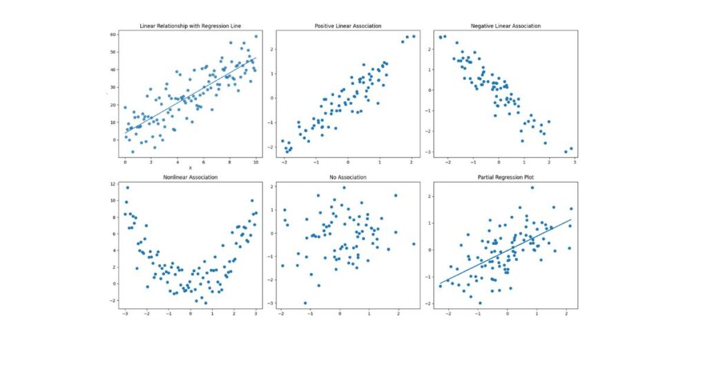
1. Bivariate Scatterplots

Plot each predictor against the dependent variable.

• A straight-line trend supports linearity
• Curves, waves, or clusters indicate violation

This step is especially important before running regression.

2. Partial Regression (Added Variable) Plots

These plots show the unique relationship between each predictor and the outcome while controlling for other predictors.

They are particularly useful in:

• Multiple regression models
• Models with correlated predictors

3. Residuals vs Fitted Values Plot

If linearity holds:

• Residuals will be randomly scattered
• No visible curvature should appear

Systematic curves signal model misspecification.

Remedies for Non-Linearity

• Apply transformations (log, square root, inverse)
• Add polynomial terms (e.g., X²)
• Use interaction effects
• Consider non-linear or generalized models

Assumption 2: Independence of Errors

What Independence Really Means

Independence of errors means that one observation’s error does not predict another’s. This assumption is most often violated in data where observations are ordered or clustered.

Common risk scenarios include:

• Time-series data
• Longitudinal designs
• Panel data
• Clustered samples (schools, hospitals, regions)

Why Independence Is Crucial

When errors are correlated:

• Standard errors become biased
• Hypothesis tests are unreliable
• Confidence intervals are distorted

Regression coefficients may appear significant when they are not.

Testing Independence

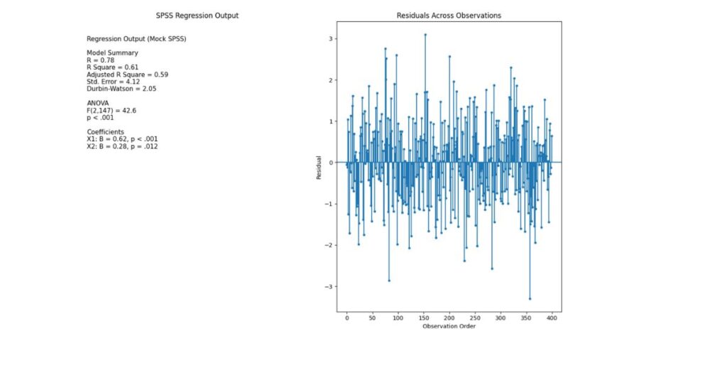
Durbin–Watson Statistic

The most widely used diagnostic for first-order autocorrelation.

• Values range from 0 to 4
• Around 2 indicates independence

Interpretation:

• <1.5 → positive autocorrelation
• 2.5 → negative autocorrelation

Graphical Diagnostics

• Plot residuals against time or order of data
• Look for repeating patterns or trends

Remedies for Autocorrelation

• Include lagged dependent variables
• Use time-series regression models
• Apply generalized least squares
• Use clustered or robust standard errors

Assumption 3: Homoscedasticity

Meaning of Homoscedasticity

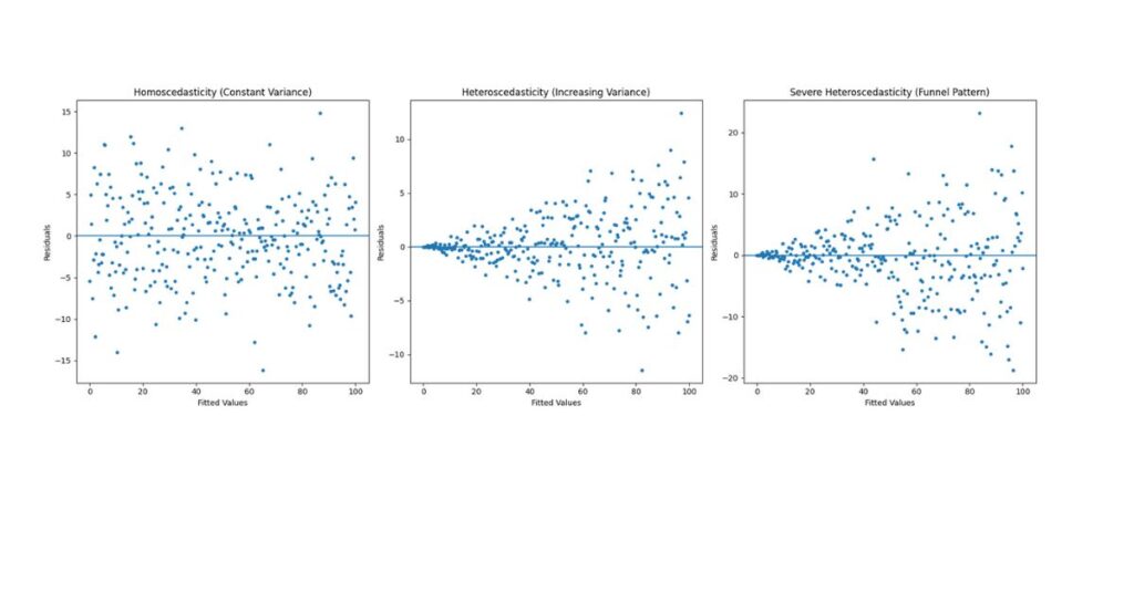
Homoscedasticity means that the variability of errors remains constant across all predicted values.

If variance increases or decreases systematically, the data are heteroscedastic.

Why Constant Variance Matters

When heteroscedasticity exists:

• Coefficient estimates remain unbiased
• Standard errors become incorrect
• p-values and confidence intervals are invalid

This is a serious threat to inference, even when R² looks strong.

How to Detect Heteroscedasticity

Residuals vs Predicted Values Plot

• Equal vertical spread → assumption met
• Funnel or cone shape → violation

Formal Statistical Tests

• Breusch–Pagan Test
• White Test

These tests assess whether residual variance depends on predictors.

How to Fix Heteroscedasticity

• Transform the dependent variable
• Use heteroscedasticity-robust standard errors
• Apply weighted least squares
• Reconsider model specification

Assumption 4: Normality of Residuals

Clarifying the Normality Assumption

Normality applies to residuals, not variables. This assumption supports:

• Valid t-tests for coefficients
• Accurate confidence intervals

Regression coefficients remain unbiased even if residuals are non-normal, but inference suffers.

Diagnostic Techniques

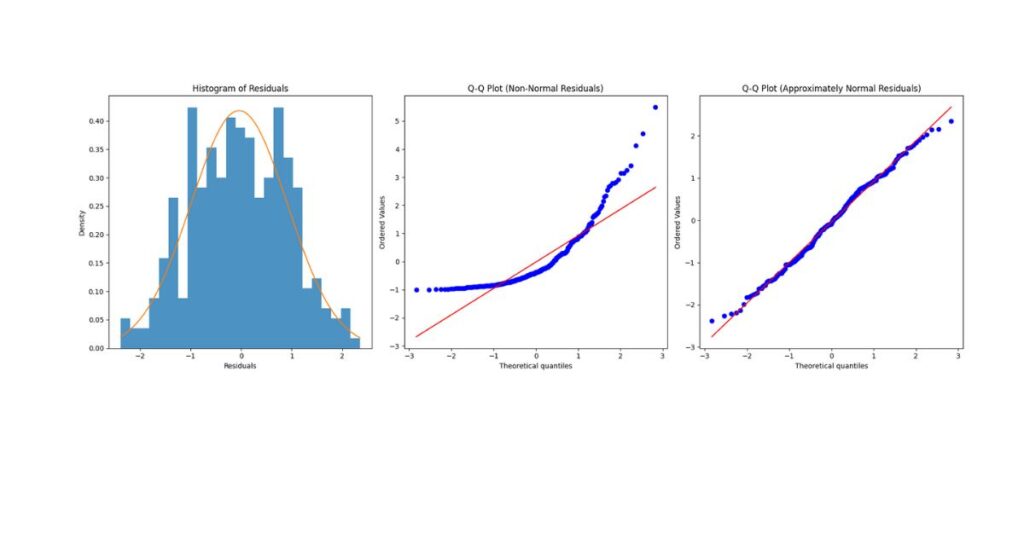
Histogram of Residuals

• Should resemble a bell curve
• Mild skewness is acceptable

Q–Q Plot

• Points should align closely with the diagonal
• Systematic deviation suggests non-normality

Statistical Tests

• Shapiro–Wilk
• Kolmogorov–Smirnov

Large samples often fail these tests even when distributions are acceptable, so visual inspection is essential.

Remedies for Non-Normality

• Transform outcome variable
• Address outliers
• Use bootstrapping
• Increase sample size

Assumption 5: No Multicollinearity

Understanding Multicollinearity

Multicollinearity occurs when predictors share excessive variance. While regression can still run, interpretation becomes unstable.

Why Multicollinearity Is Problematic

• Inflated standard errors
• Coefficients change dramatically with small data changes
• Predictors appear insignificant despite strong relationships

Diagnostic Methods

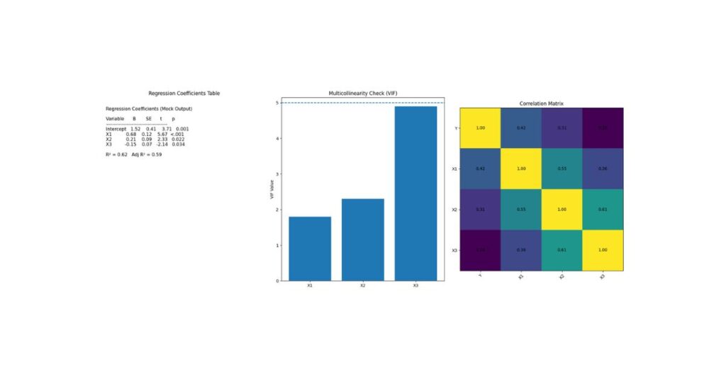
Correlation Matrix

• Correlations >0.80 are concerning

Variance Inflation Factor (VIF)

• <5 acceptable
• 5–10 moderate concern
• 10 severe problem

Solutions

• Remove redundant predictors
• Combine variables
• Center predictors
• Use dimension reduction techniques

Influential Outliers & Leverage

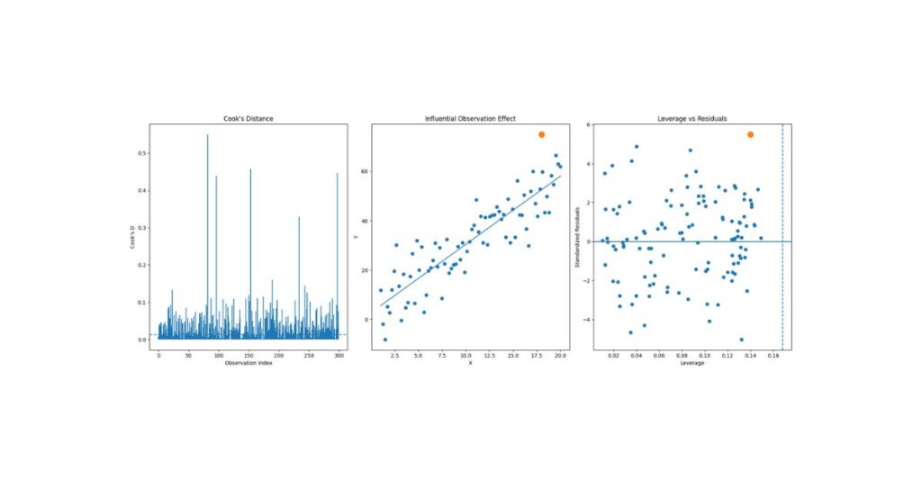
Outliers can disproportionately influence regression results.

Key Diagnostics

• Standardized residuals
• Leverage values
• Cook’s Distance

Observations with Cook’s Distance >1 require investigation.

Best Practices

• Never delete automatically
• Verify data accuracy
• Report sensitivity analyses
• Justify decisions transparently

Comprehensive Regression Assumptions Checklist

✔ Scatterplots → Linearity
✔ Durbin–Watson → Independence
✔ Residual plots → Homoscedasticity
✔ Histogram & Q–Q plot → Normality
✔ VIF → Multicollinearity
✔ Cook’s Distance → Influence

How to Report Assumptions in APA Style

Example:

Prior to analysis, assumptions of linear regression were evaluated. Visual inspection of scatterplots and partial regression plots supported linear relationships between predictors and the outcome variable. Residuals were independent (Durbin–Watson = 2.01), approximately normally distributed, and homoscedastic. Variance inflation factors ranged from 1.12 to 2.36, indicating no multicollinearity. No influential outliers were detected.

Final Thoughts

Testing regression assumptions is not a procedural formality—it is a core requirement of valid statistical reasoning. Proper diagnostics:

• Strengthen credibility
• Improve interpretability
• Protect against false conclusions
• Elevate academic quality

A well-validated regression model is far more valuable than one with impressive but unreliable statistics.