

Sample size calculation is the process of determining how many participants, records, or observations a study needs to answer its research question with an acceptable level of precision and statistical power. The correct method depends on your research design, the statistical test you plan to run, your expected effect size, your significance level, your desired power, your population, your precision requirements, and the nonresponse or attrition you expect. There is no single universal sample size formula that works for every study. A sample that is too small produces unstable, underpowered results, while a sample that is unnecessarily large wastes time, money, and participant burden without adding meaningful value.
This guide walks through every major sample size calculation formula, a full G*Power tutorial, worked examples for the most common statistical tests, and a practical framework for writing a defensible sample size justification in Chapter 3 of your dissertation.
Not sure which formula applies to your study design? Reach out for help and our team can walk you through the correct calculation for your specific hypotheses.
What Is Sample Size Calculation?
Sample size is the number of participants, cases, or units included in a study. The population is the entire group a researcher wants to draw conclusions about, for example all registered nurses in a state, or all undergraduate business students at a university. A study almost never collects data from an entire population, so researchers select a smaller, manageable group: the sample.
Sample size calculation is the statistical process used to work out, in advance, how large that sample needs to be. It is distinct from three related but different figures. The planned sample size is the target number calculated before recruitment begins. The recruited sample size is the number of people who actually enroll or respond. The final analytic sample size is the number of usable cases remaining after exclusions, missing data, and dropouts are removed.
Sample size planning should happen before data collection starts, not afterward. Calculating sample size after data has already been gathered (a practice sometimes called retrofitting) does not protect a study from being underpowered; it only describes an outcome that has already occurred.
Quick definition: Sample size calculation is the statistical process of estimating the minimum number of participants or observations a study needs, based on the planned analysis, expected effect size, significance level, desired power, and anticipated nonresponse, so that results are precise and defensible.
Why Is the Correct Sample Size Important?
Sample size influences almost every dimension of a study’s quality. It shapes statistical power, the probability of detecting a real effect if one exists, since larger samples generally increase power. It shapes precision, because larger samples produce narrower confidence intervals and more stable estimates. It affects the risk of Type I and Type II errors: an underpowered study raises the risk of a Type II error (failing to detect a real effect), while poor design choices elsewhere can raise the risk of a Type I error (a false positive). It affects generalizability, since an appropriately sized, well-sampled group supports broader conclusions about the population.
Sample size also has practical and ethical weight. Recruitment, materials, and researcher time scale with sample size, so research costs rise accordingly. Enrolling more participants than necessary, particularly in clinical or interventional research, raises unnecessary ethical exposure, while enrolling too few can waste the contributions of the participants who did take part, since the study may be unable to answer its own question. Committees and reviewers also expect a documented, defensible sample size calculation in Chapter 3, so the choice directly affects the credibility of a dissertation’s methodology.
| Sample size problem | Likely consequence |
|---|---|
| Sample too small | Low power and unstable estimates |
| Sample too large | Unnecessary cost and participant burden |
| High nonresponse | Final sample below the required minimum |
| Poor sampling method | Large but unrepresentative sample |
| Incorrect assumptions | Misleading sample size result |
A large sample cannot correct biased sampling, invalid measurement instruments, weak methodology, or incorrect statistical analysis. Sample size only addresses the amount of data collected; it does not fix how that data was collected or measured.
This article focuses on selecting, calculating, and justifying sample size. For a deeper discussion of statistical power specifically, see our power analysis in SPSS guide. For how sample size relates to the width of a confidence interval, see how sample size affects confidence intervals.
What Information Is Needed to Calculate Sample Size?
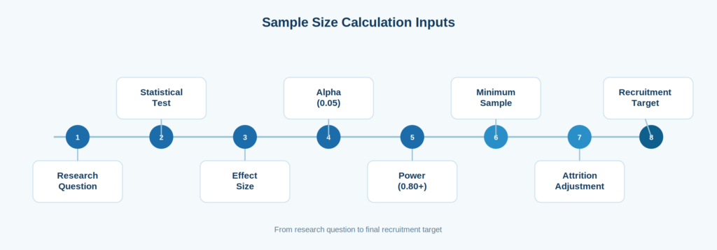
Several inputs determine which calculation method fits your study and what number it produces.
Research design. The calculation method depends heavily on design. Surveys and prevalence studies typically rely on confidence level and margin of error formulas. Experiments, comparative studies, and repeated measures designs typically rely on power analysis. Observational, correlational, and longitudinal studies often combine both approaches, depending on the specific outcome being tested.
Primary research question or outcome. Most dissertations test several relationships, but the sample size calculation should generally be built around the primary hypothesis or the single most important outcome. Calculating sample size for a secondary or exploratory analysis while ignoring the main research question is a common and avoidable error.
Planned statistical test. The required sample depends on which test will analyze the primary outcome, including the independent samples t-test, paired samples t-test, one way ANOVA, repeated measures ANOVA, correlation, multiple regression, logistic regression, chi-square test, mediation and moderation, factor analysis, and structural equation modeling. Each test has its own inputs and its own sample size logic.
Effect size. Effect size is a standardized measure of how large or meaningful a difference, relationship, or association is expected to be, independent of sample size. Effect sizes are typically described as small, medium, or large, based on conventions such as those proposed by Jacob Cohen. Wherever possible, the assumed effect size should come from prior published studies, a meta-analysis, pilot data, or a minimum effect the researcher considers practically meaningful, rather than from whatever number happens to produce a convenient sample size. Selecting an inflated effect size purely to shrink the required sample undermines the credibility of the entire calculation.
Significance level. Alpha is the threshold for statistical significance, the probability of rejecting a true null hypothesis (a Type I error). An alpha of 0.05 is the most common convention in social science, health, and business research, but it is not mandatory. Some fields, disciplines, or multiple comparison situations call for a stricter or more lenient threshold, and the choice should be justified in context.
Statistical power. Statistical power is the probability that a study will detect a real effect if one truly exists, in plain terms, the chance of avoiding a false negative. Power levels of 0.80 and 0.90 are commonly discussed in the literature, but neither is a mandatory universal standard; the appropriate power level should reflect the consequences of missing a true effect in that specific field.
Population size. For most inferential hypothesis testing designs (t-tests, ANOVA, regression), population size has very little effect on the required sample, because these tests rely on distributional assumptions rather than a finite pool of cases. Population size becomes important mainly in survey and prevalence research using a finite population correction, particularly when the accessible population is small.
Confidence level and margin of error. Confidence level reflects how confident the researcher wants to be that the true population value falls within a calculated range, commonly 90%, 95%, or 99%. Margin of error is the acceptable amount of imprecision around an estimate. These two inputs are central to descriptive surveys and proportion estimation studies, where the goal is to estimate a characteristic of a population rather than test a hypothesis.
Number of groups and predictors. Adding comparison groups, predictors, interaction terms, or repeated measurement occasions generally increases the sample required to maintain the same power, because the design must estimate more parameters or detect more specific comparisons from the same variability.
Expected response rate, attrition, and missing data. The number calculated by a formula or by G*Power represents the minimum analytic sample, the number of usable, complete cases needed. Researchers must inflate this number to account for anticipated nonresponse, dropout, incomplete surveys, unusable records, and planned exclusions, so that the final dataset still meets the minimum requirement.
Unsure which of these inputs applies to your study? Send us your research questions and design and our statistical consultants can help you identify the correct calculation approach before you commit to a method.
Sample Size Calculation Formula for Surveys
The most widely used formula for estimating a population proportion in survey and descriptive research is:
Formula: n₀ = Z²p(1 − p) / e²
Here, n₀ is the required sample size. Z is the Z-score associated with the desired confidence level (1.96 for 95% confidence). p is the estimated proportion of the population with the characteristic of interest. e is the acceptable margin of error, expressed as a decimal.
When no reliable prior estimate of p exists, researchers commonly set p = 0.50. This is because p(1 − p) is at its mathematical maximum when p equals 0.50, which produces the most conservative (largest) sample size estimate and protects against underestimating the required sample.
Worked example: Using a 95% confidence level (Z = 1.96), a 5% margin of error (e = 0.05), and p = 0.50:
Z² equals 1.96 squared, or 3.8416. p(1 − p) equals 0.50 times 0.50, or 0.25. Multiplying these gives a numerator of 3.8416 times 0.25, or 0.9604. e² equals 0.05 squared, or 0.0025. Dividing, n₀ equals 0.9604 divided by 0.0025, or 384.16.
Rounding up, the required sample size is 385 respondents. This is the well known “384” figure that appears throughout survey methodology literature, and it assumes an effectively unlimited population.
Finite Population Correction
When the accessible population is relatively small and clearly defined, the initial estimate can be adjusted downward using the finite population correction:
Formula: n = n₀ / [1 + (n₀ − 1)/N]
Here, N is the size of the accessible population and n₀ is the sample size calculated from the proportion formula above.
This correction matters most when N is small relative to n₀. For a very large or effectively unlimited population, the correction makes almost no difference. Researchers must also be careful to distinguish the realistic accessible population (for example, employees at a specific organization) from an extremely broad theoretical population (for example, “all employees worldwide”), since applying the correction to an unrealistic population figure produces a misleading result.
Worked example: Using n₀ = 385 and a defined population of N = 1,200:
n₀ minus 1 equals 384. Dividing 384 by 1,200 gives 0.32. Adding 1 gives 1.32. Dividing 385 by 1.32 gives 291.7.
The corrected required sample size is approximately 292 respondents.
Adjusting Sample Size for Nonresponse or Attrition
The sample size produced by a formula or by G*Power is the minimum required analytic sample, the number of complete, usable cases needed. Because some invited participants will not respond, and some enrolled participants will drop out, researchers should inflate their recruitment target using:
Formula: Adjusted sample = Required sample / (1 − anticipated nonresponse rate)
For a survey with a required sample of 384 and a 20% expected nonresponse rate, the adjusted sample equals 384 divided by 0.80, or 480 invitations needed.
For an experiment with a required sample of 128 (64 per group) and a 15% expected dropout rate, the adjusted sample equals 128 divided by 0.85, or roughly 151 participants to enroll.
It is important to distinguish between increasing the number of people invited or enrolled (a recruitment decision) and changing the statistical sample size requirement itself (a methodological decision). The 384 or 128 figures remain the analytic requirement; the 480 or 151 figures are the recruitment targets needed to reach that requirement after expected losses.
Sample Size Calculation Using G*Power
GPower is a free statistical software program, developed at Heinrich Heine University Düsseldorf, that calculates sample size and power for a wide range of statistical tests. Unlike the proportion based survey formula above, GPower is built around power analysis, which uses effect size, alpha, and desired power to calculate the sample needed to detect a hypothesized effect with a specific statistical test.
Running an a priori analysis in GPower follows a consistent sequence. Begin by identifying the correct test family (t-tests, F-tests, chi-square tests, z-tests, or exact tests), then select the specific statistical test that matches your planned analysis. Choose “A priori” as the type of power analysis, since this calculates sample size from effect size, alpha, and power rather than the reverse. Enter the effect size, ideally sourced from prior literature or pilot data, along with the alpha level (commonly 0.05, though you should confirm this fits your design) and the desired power (commonly 0.80 or 0.90). Add any additional design inputs, such as the number of groups, predictors, or repeated measurements, and select Calculate. GPower will report the total sample size and the actual power achieved. Finally, inflate that result for anticipated attrition or incomplete data, using the nonresponse adjustment formula above.
G*Power supports a wide range of t-tests, F-tests, chi-square tests, z-tests, and exact tests, but the software itself does not eliminate the need to choose defensible assumptions; it only performs the calculation once those assumptions are entered.
Warning: Do not manipulate the effect size, alpha, or power until G*Power produces a sample size you can conveniently recruit. Every input must have a defensible methodological justification, ideally traceable to prior literature, pilot data, or an explicitly stated minimum meaningful effect.
Unsure which test family or inputs apply to your study? Submit your research questions, hypotheses, planned analysis, number of groups or predictors, relevant prior studies, and any supervisor requirements, and our consultants can help you build a customized, defensible G*Power calculation.
Sample Size Examples for Common Statistical Tests
The examples below are illustrative only. They demonstrate how each calculation works; they are not universal recommendations for every study using that test.
Independent samples t-test. Key inputs include the expected difference between group means, the standard deviation, the standardized effect size (Cohen’s d), alpha, power, and the allocation ratio between groups. Assuming a medium effect size (d = 0.50), alpha = 0.05, power = 0.80, and equal group allocation, a G*Power a priori calculation typically indicates approximately 128 total participants, or 64 per group. This is an illustrative figure, not a fixed rule for every two group comparison.
Paired samples t-test. Paired designs compare the same participants across two conditions or time points, so the expected correlation between the repeated measurements affects the required sample. Higher correlations between paired scores generally reduce the number of participants needed to detect the same effect size, compared with an independent groups design.
One way ANOVA. Key inputs include the number of groups, the effect size f, alpha, and power. GPower reports both the total sample size and the sample size implied per group. With three groups, a medium effect size (f = 0.25), alpha = 0.05, and power = 0.80, a GPower a priori calculation typically indicates approximately 158 total participants, or roughly 53 per group.
Correlation. Key inputs include the expected correlation coefficient, alpha, power, and whether the test is one tailed or two tailed. Smaller expected correlations require substantially larger samples to detect reliably than larger expected correlations.
Multiple regression. Key inputs include the number of predictors, whether the researcher is testing the overall model (R²) or an individual predictor’s effect, the effect size f², alpha, and power. Simplistic “participants per predictor” rules, such as those attributed to Green (1991), can offer a rough starting estimate, but they should not automatically replace a properly specified power analysis, since they do not account for the actual expected effect size or model complexity.
Logistic regression. Sample size planning for logistic regression depends on outcome prevalence, the frequency of the event being predicted, the number of predictors, model complexity, and the risk of separation (a data pattern that makes some models unstable). The historical “10 events per variable” guideline is a useful starting heuristic, not an inflexible universal law; modern planning often calls for a more detailed simulation based assessment, particularly with rare outcomes.
Mediation and moderation. Testing indirect effects (mediation) or interaction effects (moderation) generally requires larger samples than testing simple main effects, because indirect and interaction effects tend to be smaller and harder to estimate precisely. Many mediation analyses rely on bootstrap confidence intervals, and formal sample size planning for these models often requires simulation based methods or specialized power software rather than a simple formula.
Factor analysis. Sample size needs for factor analysis depend on the number of items, the number of factors, the strength of communalities, the size of factor loadings, overall model complexity, and data quality. Commonly cited participant to item ratios (such as 10:1) are rough heuristics only; no single fixed ratio is appropriate for every factor analysis, since a model with strong, clean loadings can be adequately estimated with fewer cases than a model with weak or ambiguous loadings.
Structural equation modeling. Structural equation modeling (SEM) sample size requirements depend on model complexity, the number of latent variables, the number of indicators per latent variable, expected effect sizes, anticipated missing data, the estimation method, distributional assumptions, and the desired precision of fit indices. Because so many factors interact, simulation based sample size planning or expert statistical consultation is generally recommended for SEM models rather than a single fixed formula.
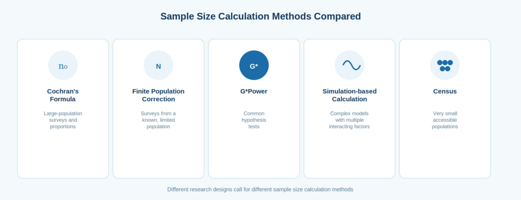
Sample Size Calculation Methods Compared
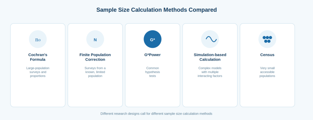
| Method | Most appropriate use | Main inputs | Key limitation |
|---|---|---|---|
| Cochran’s formula | Large population surveys or proportions | Confidence, margin of error and proportion | Not appropriate for every analytical model |
| Finite population correction | Surveys from a known, limited population | Initial sample and population size | Requires a defensible population size |
| G*Power | Common hypothesis tests | Effect size, alpha, power and design | Depends heavily on correct assumptions |
| Simulation based calculation | Complex models | Full model assumptions | Requires specialist software and expertise |
| Published rules of thumb | Preliminary planning | Test specific guideline | May ignore the actual effect and study design |
| Census | Very small accessible populations | Entire population | Nonresponse may still occur |
Cochran’s Formula Versus Slovin’s Formula
Cochran’s formula, the proportion formula presented earlier (n₀ = Z²p(1−p)/e²), is grounded in confidence level, margin of error, and an estimated or assumed proportion. It is widely used and well documented in survey methodology literature.
Slovin’s formula, n = N / (1 + Ne²), is a simplified approach that estimates sample size from population size (N) and margin of error (e) alone, without explicitly incorporating a confidence level or an estimated proportion. It is often used in student research because it is quick to apply and requires only two known values.
Slovin’s formula can be more difficult to justify in a dissertation methodology chapter because its underlying statistical assumptions are less explicitly stated than Cochran’s formula, and it does not directly incorporate confidence level or an assumed population proportion. This does not mean students or supervisors who use it have made an error; it means that whichever formula is chosen, the researcher should clearly state its assumptions and explain why it fits the study’s research question and planned analysis.
Does SPSS Calculate Sample Size?
SPSS is primarily used for statistical analysis after or during data collection, not for a priori sample size calculation. Standard SPSS Statistics menus do not include comprehensive a priori sample size and power analysis tools for most designs. Sample size and power planning is typically conducted using G*Power, IBM SPSS SamplePower (a separate, specialized add on module where licensed and available), other dedicated software such as R, Stata, or PASS, published formulas, or simulation methods.
It is worth distinguishing between several related but different concepts. SPSS is general purpose statistical analysis software. G*Power is dedicated software for a priori and post hoc power and sample size calculations. Power analysis is the broader statistical method of relating effect size, alpha, power, and sample size. Sample size calculation is the specific output, a number of participants, derived from that method. Post hoc power is power calculated after data collection, based on the effect actually observed; this is generally discouraged as a substitute for a priori planning, since it largely restates the study’s p-value in different terms.
How to Justify Sample Size in a Dissertation
A strong Chapter 3 sample size justification should clearly state the primary statistical test or research objective, the type of sample size calculation used, the software or formula applied, the assumed effect size and its source, the significance level, the desired power, the number of groups or predictors, the minimum required sample, the allowance for nonresponse or attrition, and the final recruitment target.
Methodology paragraph template:
“An a priori power analysis was conducted using [software] to determine the minimum sample required for [statistical test]. Assuming an effect size of [value], an alpha level of [value], statistical power of [value], and [number] predictors/groups, the analysis indicated that at least [number] participants were required. To account for an anticipated [percentage]% rate of nonresponse or attrition, the recruitment target was increased to [number].”
Every placeholder must be replaced with values that are justified by your own study design, prior literature, and pilot data; the template is a structure to build from, not a finished sentence.
Common Sample Size Calculation Mistakes
| Mistake | Correction |
|---|---|
| Calculating sample size before identifying the primary analysis | Confirm the primary hypothesis and test first |
| Using the wrong statistical test in G*Power | Match the test family to your actual planned analysis |
| Selecting an effect size without evidence | Source it from literature, pilot data, or a stated minimum meaningful effect |
| Choosing a larger effect solely to reduce sample size | Base the effect size on evidence, not convenience |
| Confusing population size with sample size | Clarify which figure the calculation actually requires |
| Ignoring response rate or attrition | Apply the nonresponse adjustment formula |
| Treating 30 participants as universally sufficient | Base the number on a calculation specific to your design |
| Applying one formula to every type of research | Match the method to the research design and test |
| Using a rule of thumb without justification | State why the heuristic fits your specific study |
| Confusing per group and total sample size | Report both figures clearly in your methodology |
| Using post hoc power as a substitute for planning | Conduct a priori power analysis before data collection |
| Ignoring unequal group allocation | Adjust the calculation for the planned allocation ratio |
| Ignoring missing data and exclusion criteria | Build expected exclusions into the recruitment target |
| Recruiting a convenient sample and calculating afterward | Plan the sample size before recruitment begins |
| Believing a large sample fixes poor quality data | Address sampling and measurement quality independently |
What If You Cannot Reach the Required Sample Size?
If recruitment challenges make the calculated sample size unreachable, several responsible options exist. You can reconsider the scope of the research question, focus on a smaller number of primary hypotheses, or use a repeated measures design where theoretically appropriate. You can improve measurement precision, use more efficient or targeted recruitment methods, extend the recruitment period, or collaborate with additional sites or partners. You can also reassess unrealistic effect size or attrition assumptions, conduct a feasibility or pilot study first, clearly report the limitation in the dissertation, and consult a statistician before changing the design.
Reducing methodological rigor simply to reach a smaller, more convenient number is not an appropriate solution and can undermine the credibility of the entire study.
Sample Size Calculation Checklist
Before data collection begins, confirm that the primary outcome is identified, the research hypothesis is finalized, and the planned statistical analysis is selected. Confirm that the effect size is justified, alpha is selected, and power is selected. Confirm the number of groups or predictors, and that the allocation ratio has been considered. Confirm that attrition or nonresponse has been estimated, that the minimum analytic sample and the recruitment target have both been calculated, that every assumption is documented, and that a supervisor or statistician has reviewed the calculation.
When to Consult a Dissertation Statistician
Expert statistical support is particularly useful when a study involves multiple primary outcomes, mediation or moderation, multilevel or clustered data, repeated measurements, unequal group sizes, logistic regression with rare outcomes, complex survey designs, factor analysis, structural equation modeling, missing data, longitudinal follow up, clinical trial requirements, or limited prior evidence for estimating an effect size.
These situations do not mean a student has done anything wrong. They simply involve more moving parts than a single formula or a basic G*Power calculation can resolve on its own, and a second, experienced set of eyes can help confirm that every assumption is defensible before data collection begins.
If your study involves any of the situations above, our dissertation statistics consultant can review your design and help you build a sample size calculation your committee will find credible.
Frequently Asked Questions
Sample size calculation is the statistical process of determining how many participants or observations a study needs. It considers the planned statistical test, expected effect size, significance level, desired power, and anticipated nonresponse or attrition, and it should be completed before data collection begins.
Start by identifying your primary research question and the statistical test that will analyze it. Then gather your assumed effect size, alpha, and power (or your confidence level and margin of error for a survey), and use the matching formula or G*Power to calculate the minimum required sample, adjusting afterward for expected nonresponse.
There is no single minimum that applies to every quantitative study. The required minimum depends on the planned statistical test, the expected effect size, the desired power, and the study design, and must be calculated individually for each research project.
Not necessarily. Thirty is sometimes cited informally as a rough threshold for normal distribution assumptions, but it is not a validated sample size calculation for any specific statistical test. The correct number depends on your effect size, alpha, power, and design.
For most inferential tests (t-tests, ANOVA, regression), population size has little practical effect on the required sample. It becomes relevant mainly in survey research through the finite population correction, particularly when the accessible population is small.
Confidence levels of 90%, 95%, and 99% are common conventions, with 95% used most frequently in social science and health research. The appropriate level depends on how much precision your research question requires and the norms of your specific field.
Power levels of 0.80 and 0.90 are frequently used in published research, but neither is a mandatory standard. The appropriate power level should reflect how costly it would be to miss a real effect in your particular study.
Choose an effect size based on prior published studies, a meta-analysis, pilot data from your own research, or a minimum effect you consider practically meaningful. Avoid selecting a larger effect size simply because it produces a smaller, more convenient sample size.
Standard SPSS Statistics menus do not provide comprehensive a priori sample size calculation for most designs. Sample size and power analysis are typically performed using G*Power, a specialized SPSS add on module where available, or other dedicated software such as R, Stata, or PASS.
Select the correct test family and statistical test, choose “A priori” analysis, enter your effect size, alpha, and desired power, add any group or predictor information, and select Calculate. G*Power will report the total required sample size and the actual power achieved.
Both figures matter. G*Power and most formulas report a total sample size, which should then be divided according to your allocation ratio to confirm the number required per group, especially in unequal allocation designs.
Divide your minimum required analytic sample by (1 minus your anticipated nonresponse or attrition rate). This produces the number of participants you need to invite or enroll to end up with enough complete, usable cases.
Consider narrowing your research question, extending your recruitment timeline, improving recruitment strategy, collaborating across additional sites, or reassessing your assumptions, and report any resulting limitation transparently. Consult a statistician before changing your design.
Cochran’s formula incorporates confidence level, margin of error, and an estimated population proportion. Slovin’s formula estimates sample size from population size and margin of error alone, without an explicit confidence level or proportion, which can make its assumptions harder to state explicitly in a methodology chapter.
No. A larger sample increases precision and power, but it cannot correct a biased sampling method, an invalid measurement instrument, a flawed research design, or an incorrect statistical analysis.
State the statistical test, the software or formula used, the assumed effect size and its source, the alpha level, the desired power, the number of groups or predictors, the resulting minimum sample, and the adjusted recruitment target after accounting for nonresponse or attrition.
Conclusion
An appropriate sample size calculation depends on your specific research question, planned statistical test, expected effect, desired power, required precision, target population, and overall study design; there is no single formula that fits every project. The most defensible dissertations calculate and document their sample size before data collection begins, using assumptions that are grounded in evidence rather than convenience.
If you are unsure which calculation method fits your study, how to run or interpret a G*Power analysis, how to justify your effect size, how to adjust for attrition, or how to write your Chapter 3 sample size justification, our team at SPSSDissertationHelp.com can help. We also support the eventual SPSS analysis once your data collection is complete, and we can help you respond to supervisor or committee feedback on your methodology. Contact us to discuss your research design and recruitment plan.
