Bayesian Statistics in SPSS: A Complete Practical Guide

Many dissertation researchers reach a comfortable working knowledge of p-values, confidence intervals, and significance testing, and then a supervisor or reviewer asks them to report a prior, a posterior distribution, a Bayes factor, or a Bayesian credible interval instead. At that point, the familiar SPSS output screen suddenly looks unfamiliar.

Yes, selected Bayesian statistical analyses can be conducted through IBM SPSS Statistics using the Bayesian Statistics procedures. However, researchers must choose an appropriate model, justify the prior, understand the direction of the Bayes factor, and interpret the posterior output correctly. Selecting a menu option is the easy part; defending the choices behind it is what a dissertation committee will actually examine.

This guide works through the full process: what Bayesian statistics means, which procedures SPSS actually supports, how to run a complete worked example from data entry to APA 7 write-up, how to interpret every part of the output, and where SPSS’s native Bayesian tools reach their limits. If your project needs professional SPSS data analysis support, the same principles covered here, transparent priors, correct model selection, and honest reporting, are exactly what a good analyst applies to your data.

Key takeaways

• SPSS supports a defined set of native Bayesian procedures, not every Bayesian model.
• A Bayes factor compares evidence for two models; it is not a probability that a hypothesis is true.
• The prior must be chosen and justified before looking at the results, not adjusted afterward to strengthen a conclusion.
• A credible interval and a confidence interval answer different questions and should not be described as interchangeable.

What Is Bayesian Statistics?

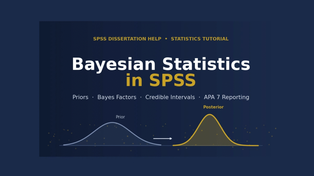
Bayesian statistics is an approach to inference in which an unknown parameter is represented using a probability distribution rather than a single fixed value. Existing knowledge or assumptions about the parameter are expressed as a prior distribution. This prior is then combined with the likelihood of the observed data to produce a posterior distribution, which becomes the basis for estimation, interval statements, and model comparison.

The general form of Bayes’ theorem is:

P(θ | data) ∝ P(data | θ) × P(θ)

• P(θ | data): the posterior distribution, what is believed about the parameter after seeing the data
• P(data | θ): the likelihood, how compatible the data are with different parameter values
• P(θ): the prior distribution, what was believed before seeing the data
• θ: the unknown population parameter (for example, a mean difference)
• ∝: proportional to

A simple everyday analogy: if you believe a coin is probably fair (your prior), and you then observe 80 heads out of 100 flips (your data), your updated belief about the coin’s fairness (your posterior) shifts toward “probably biased.” How far it shifts depends on how strong your original belief was and how much data you collected.

Applied to dissertation research, consider a researcher investigating whether a mindfulness intervention reduces academic stress. The researcher starts with some prior assumption about the plausible size of the effect, perhaps informed by earlier meta-analyses, and updates that assumption using the stress scores actually collected. The posterior distribution then summarizes the credible range of effect sizes given both sources of information.

The Prior Distribution

The prior represents what is assumed about a parameter before the current data are analyzed. It can come from earlier published studies, pilot data, established theory, or plausible-range judgment from subject-matter expertise.

• Informative priors encode specific, defensible expectations (for example, an effect size range from a prior meta-analysis).
• Weakly informative priors rule out implausible extremes without asserting a specific value.
• Noninformative or reference priors attempt to let the data dominate the conclusion, though a so-called noninformative prior still embeds mathematical assumptions and is not truly assumption-free.
• Conjugate priors are chosen because they combine mathematically with a particular likelihood to produce a posterior from the same distribution family (for example, a Beta prior with a Binomial likelihood).

Priors must be selected and documented before the analysis is run, and the justification should be stated explicitly in the write-up. Changing a prior after seeing disappointing output, purely to obtain a stronger Bayes factor, undermines the integrity of the analysis.

The Likelihood

The likelihood expresses how compatible different candidate parameter values are with the data actually observed, given the chosen statistical model. It is not simply “the data”; it is a function that links the data to each possible parameter value. Importantly, the likelihood tells you the probability of the data given a hypothesis. It does not tell you the probability that the hypothesis itself is true.

The Posterior Distribution

The posterior combines the prior and the likelihood into a single distribution that expresses the most credible parameter values along with remaining uncertainty. It communicates direction, magnitude, and a range of plausible values simultaneously, more information than a single point estimate and interval computed under repeated-sampling logic. The posterior is always conditional on the observed data, the chosen likelihood, the prior, and the assumptions of the model. Change any of those and the posterior changes too.

Bayesian Credible Intervals

A 95% credible interval is the range within which the parameter is believed to lie with 95% probability, conditional on the model, the data, and the prior used. This differs fundamentally from a frequentist confidence interval, which is not normally interpreted as a direct probability statement about where the fixed population parameter lies; instead, it describes long-run coverage across repeated samples. A credible interval should never be labeled a “Bayesian confidence interval” without explaining this distinction.

Bayes Factors

A Bayes factor compares how well two competing models, typically a null and an alternative, predict the observed data.

• BF₁₀ expresses evidence for the alternative model relative to the null.
• BF₀₁ expresses evidence for the null model relative to the alternative.
• The two are reciprocals: BF₀₁ = 1 ÷ BF₁₀.

A Bayes factor is not a posterior probability, and it is not a p-value. It is a ratio of relative predictive performance between two specified models, conditional on the priors used for each.

Bayes factor interpretation (based on IBM SPSS documentation, Jeffreys 1961, and Lee and Wagenmakers 2013):

BF₁₀	Evidence category	BF₁₀	Evidence category
Greater than 100	Extreme evidence for H₁	1/3 to 1	Anecdotal evidence for H₀
30 to 100	Very strong evidence for H₁	1/10 to 1/3	Moderate evidence for H₀
10 to 30	Strong evidence for H₁	1/30 to 1/10	Strong evidence for H₀
3 to 10	Moderate evidence for H₁	1/100 to 1/30	Very strong evidence for H₀
1 to 3	Anecdotal evidence for H₁	Less than 1/100	Extreme evidence for H₀
1	No evidence either way

These labels are conventions intended to aid communication, not mechanical decision rules. Always state whether a reported value is BF₁₀ or BF₀₁, since the interpretation reverses between the two.

Prior Sensitivity Analysis

A sensitivity analysis reruns the model under several defensible priors, for example the primary prior, a weaker version, and a more concentrated but still plausible version, to check whether the Bayes factor, posterior estimate, credible interval, and practical conclusion remain stable. Reporting this analysis demonstrates that the conclusion does not depend on one arbitrary prior choice.

Bayesian Statistics Versus Frequentist Statistics

Feature	Bayesian approach	Frequentist approach
Meaning of probability	Degree of belief about a parameter	Long-run frequency across repeated samples
Use of prior information	Explicit and required	Not formally incorporated
Primary inferential output	Posterior distribution	Point estimate and p-value
Interval estimate	Credible interval (direct probability statement)	Confidence interval (repeated-sampling coverage)
Hypothesis evidence	Bayes factor (relative model support)	p-value (probability of data under H₀)
Evidence for the null	Directly quantifiable (BF₀₁)	Cannot be directly quantified by a p-value
Dependence on modelling choices	Prior and likelihood both specified	Likelihood and test assumptions specified
Common software output	Posterior mean or median, credible interval, Bayes factor	Test statistic, p-value, confidence interval

Several common misunderstandings are worth stating plainly. A p-value is not the probability that the null hypothesis is true, and it is not the probability that the observed result occurred by chance alone. Failing to reject H₀ is not automatic evidence in favor of H₀. A Bayes factor can quantify evidence for the null model directly, which a p-value cannot do. A 95% confidence interval is not generally interpreted as a 95% probability that the fixed population parameter falls within that specific interval. Bayesian results still depend on the chosen prior, likelihood, and model; they are not assumption-free.

Is Bayesian Analysis Better Than Frequentist Analysis?

Neither approach is universally superior. The right choice depends on the research question, disciplinary convention, supervisor or journal expectations, whether credible prior information exists, model complexity, sample size, and what kind of statement the researcher needs to make. Both approaches can be misapplied, and neither one compensates for poor measurement, biased sampling, weak study design, or an inappropriate model.

Can You Perform Bayesian Statistics in SPSS?

SPSS provides a dedicated Bayesian Statistics menu covering a defined set of procedures, first introduced in SPSS Statistics version 25 and expanded in later releases. It does not support every possible Bayesian model, and availability depends on the SPSS edition and licensed options. Native Bayesian procedures generally require Standard Edition or the Advanced Statistics option; some procedures are bundled with Custom Tables and Advanced Statistics.

SPSS Bayesian procedure	Suitable research question	Required variables	Key output
One Sample Normal	Compare a sample mean to a fixed value; paired-sample comparison	One or more scale test variables	Posterior estimate, credible interval, Bayes factor
Related Samples Normal	Compare two related or paired measurements	Paired scale variables	Posterior mean difference, Bayes factor
Independent Samples Normal	Compare two unrelated groups	Scale outcome plus a two-group variable	Posterior mean difference, credible interval, Bayes factor
Binomial	Estimate or test a proportion	Binary outcome	Posterior proportion, credible interval
Poisson	Analyze event counts	Count outcome	Posterior rate, credible interval
Pearson Correlation	Association between two scale variables	Two scale variables	Posterior correlation estimate, Bayes factor
One-Way ANOVA	Compare three or more independent groups	Scale outcome plus a categorical factor	Posterior group estimates, Bayes factor
One-Way Repeated Measures ANOVA	Compare repeated conditions or time points	Repeated scale measurements	Posterior estimates by condition
Linear Regression	Predict a scale outcome from predictors	Scale outcome plus predictors	Posterior coefficients, credible intervals

Do not assume SPSS natively supports Bayesian logistic regression, multilevel modeling, structural equation modeling, mediation, moderation, survival analysis, or meta-analysis unless current IBM documentation explicitly confirms it for your version.

Where Is Bayesian Statistics Located in SPSS?

The general menu path is:

Analyze > Bayesian Statistics

From there, select the submenu matching the design, such as One Sample Normal, Independent Samples Normal, Related Samples Normal, Linear Regression, or One-Way ANOVA. Menu wording can vary slightly between versions, so confirm the exact labels in your installed release.

How to Choose the Correct Bayesian Procedure

Research objective	Data structure	Recommended SPSS procedure
Compare a sample mean with a fixed value	One scale outcome	One Sample Normal
Compare two measurements from the same participants	Two related scale measurements	Related Samples Normal
Compare two unrelated groups	Scale outcome plus a two-group variable	Independent Samples Normal
Estimate a binary proportion	Binary outcome	Binomial
Analyze an event count	Count outcome	Poisson
Examine association between two scale variables	Two scale variables	Pearson Correlation
Compare three or more independent groups	Scale outcome plus a categorical factor	One-Way ANOVA
Compare repeated conditions or time points	Repeated scale measurements	One-Way Repeated Measures ANOVA
Predict a scale outcome	Scale outcome plus predictors	Linear Regression

Choosing a procedure purely by test name, without checking the data structure and independence assumptions, is a common source of avoidable analytical errors.

Preparing Data for Bayesian Analysis in SPSS

Bayesian procedures do not remove the need for careful data preparation. Before analysis, confirm one row per observational unit, correctly labeled variables and values, correct measurement levels, defined missing-value codes, correctly coded groups, and any necessary composite scores or reverse scoring. Check for duplicate cases, impossible values, outliers, and data-entry errors, and confirm the outcome type genuinely fits the chosen procedure.

If your dataset needs attention before you get to modelling, it is worth reviewing our guidance on how to clean data in SPSS first.

It also helps to distinguish between data that are missing completely at random, missing at random, and missing not at random, since the missing-data mechanism affects whether a Bayesian model’s results remain valid. Always check how the selected SPSS procedure handles missing cases for your specific design.

How to Perform Bayesian Statistics in SPSS

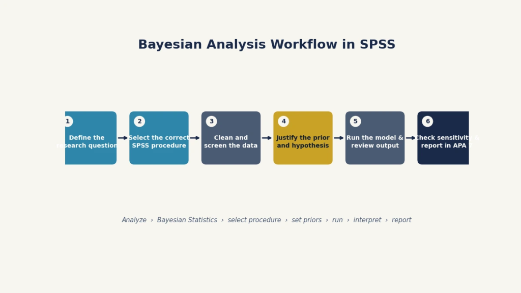
Define the research question precisely, then identify the outcome and explanatory variables and determine whether observations are independent or related. Select the correct probability model, clean and code the dataset, and specify the null and alternative models. Select and justify a prior, choose posterior characterization, Bayes-factor estimation, or both, and set the credible interval level. Request the relevant plots and statistics, run the model, and check the output carefully. Conduct a prior-sensitivity analysis, interpret magnitude and uncertainty together, and report the analysis transparently.

Each stage matters. Skipping the sensitivity check or the assumption review is one of the most common ways a Bayesian analysis becomes indefensible at a viva or peer review, even when the menu clicks were correct.

Worked Example: Bayesian Independent Samples Analysis in SPSS

The following example uses fictional, illustrative data for demonstration purposes only. It is not drawn from a real study.

Study Scenario

A researcher wants to compare academic-stress scores between students who completed a six-week mindfulness intervention and students in a waitlist control group.

• stress_score: continuous academic-stress score
• group: 1 = mindfulness intervention, 2 = control group

Research Question

Do academic-stress scores differ between students who completed the mindfulness intervention and students in the control group?

Hypotheses

• H₀: The mean stress score is equal across the two groups.
• H₁: The mean stress score differs between the two groups.

Bayesian analysis compares evidence for these two models directly rather than applying only a reject or fail-to-reject rule.

Step 1: Structure the Dataset

Participant ID	Group	Stress score
001	1	(illustrative)
002	2	(illustrative)
003	1	(illustrative)

Screenshot: SPSS Data View showing correctly structured columns for ID, group, and stress score. Screenshot: SPSS Variable View showing measurement levels and value labels for the group variable.

Step 2: Screen the Data

Check for missing cases, incorrect group codes, descriptive statistics, extreme values, and approximate normality within each group. Bayesian normal inference still relies on the outcome reasonably approximating a normal model, or a defensible approximation of one.

Step 3: Open the Bayesian Procedure

From the menus: Analyze > Bayesian Statistics > Independent Samples Normal.

Screenshot: Opening the Bayesian Statistics menu. Screenshot: Selecting the Independent Samples Normal procedure.

Step 4: Assign the Variables

Assign stress_score as the test variable and group as the grouping variable, then define the two group codes (1 and 2).

Screenshot: Assigning the test and grouping variables. Screenshot: Defining the two group codes.

Step 5: Select the Bayesian Analysis Type

SPSS offers Characterize Posterior Distribution, Estimate Bayes Factor, or Use Both Methods. For a dissertation reporting both an effect estimate and a strength-of-evidence statement, Use Both Methods is generally the most complete choice, since it produces the posterior mean difference and credible interval alongside the Bayes factor.

Screenshot: Selecting the Bayesian analysis type.

Step 6: Specify the Hypothesis Direction

Decide whether the alternative is two-sided, or directional, predicting specifically higher or lower stress in one group. This choice must follow from the theoretical or preregistered hypothesis, never from a glance at the observed group means.

Step 7: Choose and Justify the Prior

Select the prior for the effect, for example a default or reference prior scaling option, or an informed prior derived from a previous meta-analysis of mindfulness-intervention effect sizes if one is available. State explicitly which parameter receives the prior, why it is appropriate, whether it is informative or weakly informative, and what range of effects it treats as plausible. Do not select a prior after viewing the output in order to strengthen the Bayes factor.

Screenshot: Configuring the prior settings.

Step 8: Select the Credible Interval

A 95% credible interval is the conventional default unless the research protocol specifies otherwise.

Screenshot: Selecting the credible interval percentage.

Step 9: Request Relevant Plots

Where supported by the procedure and version, request plots that help assess posterior location, spread, and the credible interval range.

Screenshot: Requesting posterior plots.

Step 10: Run the Analysis

Run the procedure, then save the dataset, the output file, any generated syntax, the prior specification, the SPSS version, and the date of analysis. Recording these details is what allows the analysis to be reproduced, a requirement most dissertation committees expect even when it is not stated explicitly.

Screenshot: Reviewing the Bayes-factor output. Screenshot: Reviewing the posterior estimate. Screenshot: Interpreting the posterior distribution plot.

How to Interpret Bayesian SPSS Output

Case Processing and Sample Information

Check the number of valid cases, any excluded observations, and group sizes, since these affect how much weight the data carry relative to the prior.

Descriptive Statistics

Review the mean, standard deviation, and sample size for each group, and note the observed mean difference. A visible difference in sample means does not by itself constitute strong evidence for a population-level difference; that judgment depends on the Bayes factor and posterior distribution.

Prior Information

Confirm the prior family, its parameters, and the hypothesis values used, since these details must always be reported alongside the results.

Bayes Factor

Suppose the output reports an illustrative value of BF₁₀ = 6.40. The correct interpretation is that the observed data are approximately 6.4 times more compatible with the specified alternative model than with the specified null model, given the chosen prior and model assumptions.

The following interpretations are incorrect and should never appear in a dissertation:

• “There is a 6.4% probability that H₁ is true.”
• “The alternative hypothesis is 6.4% true.”
• “The result is statistically significant.”
• “The alternative hypothesis has been proven.”

If instead the output reports BF₀₁ = 4.00, this means the data are four times more compatible with the null model than with the alternative, under the same priors. Remember that BF₀₁ = 1 ÷ BF₁₀.

Posterior Estimate

Review the posterior mean, median, and standard deviation for the estimated mean difference, keeping the discussion tied to the actual stress-score example rather than switching to unrelated variables mid-interpretation.

Credible Interval

Suppose a fictional, illustrative 95% credible interval for the mean difference is 1.2 to 8.6. This range lies entirely above zero, suggesting a credible positive difference between groups under the specified model. An interval that contains zero, by contrast, does not itself prove there is no effect; it should be read together with the Bayes factor, the posterior distribution, the prior used, and the practical size of the estimate, not treated as a stand-alone decision rule.

Posterior Distribution Plot

Examine the plot’s central location, spread, shape, and how much of the distribution sits on either side of the null value. Posterior distributions are not always symmetric or normally shaped, so inspect the shape rather than assuming it.

Statistical Evidence Versus Practical Importance

A large Bayes factor indicates strong relative evidence between models; it does not automatically mean the effect is practically, clinically, or educationally important. Practical importance depends on the actual magnitude of the estimated effect relative to a meaningful threshold in that field, not on the strength of the evidence category alone.

Conducting a Prior Sensitivity Analysis in SPSS

Rerun the model using the primary defensible prior, a weaker prior, and a more concentrated but still plausible prior, then compare results:

Prior specification	Bayes factor	Posterior estimate	95% credible interval	Conclusion
Primary prior
Weaker prior
Stronger prior

A conclusion is considered more robust when reasonable prior variation does not materially change the direction, magnitude, interval, or evidence category of the result. If the conclusion does change substantially across plausible priors, report this openly rather than selecting whichever prior produces the strongest evidence.

How to Report Bayesian Results in APA 7

An APA-style paragraph should identify the procedure used, the SPSS version, the prior specification, whether BF₁₀ or BF₀₁ is reported, the Bayes factor value, the posterior estimate, the 95% credible interval, the practical interpretation, and the outcome of the sensitivity analysis. Use cautious language such as “the data provided moderate evidence,” “the posterior distribution suggested,” or “the conclusion was stable across the sensitivity analyses.” Avoid language such as “H₁ was accepted,” “H₀ was proven,” or describing Bayesian evidence as “statistically significant.”

Bayesian Reporting Checklist

Research question, statistical model, SPSS version, procedure, prior family and parameters, hypothesis direction, Bayes-factor notation and value, posterior estimate, credible interval, sensitivity-analysis outcome, practical importance, model assumptions, and limitations.

Already have SPSS output but are not sure how to turn it into an APA-style paragraph? A Chapter 4 data-analysis review can walk through exactly this kind of interpretation before submission.

Other Bayesian Analyses Available in SPSS

Bayesian One-Sample Normal Inference compares a sample mean (or a paired difference) against a fixed reference value, useful, for example, when testing whether a post-intervention score differs from a known benchmark.

Bayesian Related-Samples Normal Inference is for paired or repeated observations, such as before-and-after designs, and must never be analyzed as if the two measurements were independent groups.

Bayesian Independent-Samples Normal Inference is summarized in the worked example above for comparing two unrelated groups.

Bayesian Binomial Inference applies to binary outcomes with a fixed number of trials, such as the proportion of students completing a program, and can use a Beta prior for the success probability.

Bayesian Poisson Inference applies to count data such as the number of support requests received per week, typically using a Gamma prior for the event rate. Be cautious of overdispersion, which can make a simple Poisson model unsuitable.

Bayesian Pearson Correlation estimates the population correlation between two scale variables using both a Bayes factor and a posterior estimate, and, as with any correlation analysis, does not establish causation.

Bayesian One-Way ANOVA compares three or more independent groups but does not, by itself, identify which specific groups differ; follow-up comparisons are needed for that.

Bayesian One-Way Repeated-Measures ANOVA is appropriate when the same participants are measured across multiple conditions or time points, since an ordinary between-groups ANOVA would ignore the within-subject dependence.

Bayesian Linear Regression estimates posterior distributions for regression coefficients and can incorporate continuous predictors, with the same caution as any regression: coefficients from observational data do not establish causality. See our SPSS regression analysis help for the frequentist counterpart of this procedure.

Assumptions of Bayesian Analysis in SPSS

Bayesian methods are not assumption-free. Data assumptions include correct measurement levels, correctly identified independent or related observations, appropriate outcome type, reliable measurement, and sound missing-data handling. Distributional assumptions vary by model: a normal, binomial, or Poisson likelihood must reasonably represent how the data were generated. Prior assumptions concern the chosen prior family, its parameters, and the plausible range it implies. Model-specification assumptions cover correct variable choice, appropriate functional form, and issues such as outliers, overdispersion, or multicollinearity in regression. A misspecified model can produce a misleading posterior no matter how carefully the priors were chosen.

When Bayesian Statistics Are Useful in Dissertation Research

Bayesian methods are particularly useful for quantifying evidence for competing hypotheses, including evidence favoring the null, incorporating credible prior research into a current analysis, making direct probability statements about plausible parameter ranges, and supporting decision-making under uncertainty in psychology, education, nursing, public health, business, and social-science research.

Bayesian analysis does not create information that is absent from the data. With a small sample, the prior may exert more influence, and uncertainty may remain substantial. Bayesian methods do not automatically solve small-sample limitations; they simply make the influence of prior assumptions explicit.

Common Mistakes in Bayesian SPSS Analysis

Mistake	Why it is a problem	Correct approach
Confusing BF₁₀ with BF₀₁	Reverses the direction of the conclusion	Always state which ratio is reported
Treating a Bayes factor as a probability	Bayes factors compare models, not probabilities of truth	Interpret as relative predictive support
Selecting a prior without justification	Undermines transparency and reproducibility	Justify the prior before running the model
Changing the prior to get a preferred result	Introduces bias into the conclusion	Fix priors in advance; report sensitivity separately
Ignoring prior sensitivity	Conclusion may rest on one arbitrary choice	Rerun with alternative plausible priors
Treating weak evidence as evidence of no effect	A BF near 1 means the data are inconclusive, not that there is no effect	Report as inconclusive
Interpreting a credible interval as a confidence interval	The two have different logical meanings	Clarify the probability interpretation used
Ignoring practical importance	Strong evidence does not guarantee a meaningful effect size	Discuss magnitude alongside evidence
Confusing BIC with a Bayes factor	BIC is a model-selection criterion, not a directly calculated Bayes factor	Use a properly estimated Bayes factor
Using an unsupported procedure	SPSS does not natively support every Bayesian model	Confirm support in current IBM documentation
Failing to report the SPSS version	Menu options and output can vary across versions	State version, edition, and analysis date

Do not confuse BIC with a Bayes factor. The Bayesian Information Criterion is a model-selection criterion, not identical to a directly calculated Bayes factor, and the two should not be treated as automatically interchangeable.

Do not interpret inconclusive evidence as no effect. A Bayes factor close to one indicates that the data do not clearly discriminate between the two models being compared. It does not establish equivalence, prove the null, or mean the study failed.

Troubleshooting Bayesian Statistics in SPSS

Why is Bayesian Statistics missing from my SPSS menu? Possible causes include an older SPSS version (native Bayesian procedures require version 25 or later), a licensing edition that does not include the required option, or a different installation type. Check your license and the current IBM documentation for your version.

Why can’t I select my variable? Common causes are a string variable, an incorrect measurement level, an unsupported outcome type for the chosen procedure, or an improperly coded grouping variable. Verify the exact variable requirements for the specific procedure you are using.

Why is my Bayes factor extremely large? This can reflect genuinely strong data-model compatibility, a large sample size, well-separated groups, or the specific prior used, but it can also flag a coding error or outlier problem, so check the data before accepting the result at face value.

Why does the result change when I change the prior? This is prior sensitivity, and it is expected to some degree. The question is whether the revised prior is genuinely defensible on its own merits, not just convenient.

Why is my credible interval very wide? Wide intervals typically reflect a small sample, noisy measurement, high variability, a broad prior, or a model that does not fit the data well.

Why does SPSS not support my Bayesian model? SPSS’s native Bayesian menu covers a defined, limited set of procedures. For more flexible or hierarchical Bayesian models, researchers sometimes turn to specialist tools such as JASP, R, Stan, or Mplus, worth knowing about, though not a substitute for confirming what your own SPSS license already supports.

Limitations of Bayesian Analysis in SPSS

SPSS’s Bayesian toolkit is genuinely useful for the models it covers, but it has real boundaries: a limited range of native Bayesian procedures, licensing requirements for some options, less flexibility than specialist Bayesian programming environments, restricted prior choices for certain procedures, and fewer advanced diagnostics than dedicated Bayesian software. It also depends heavily on correct prior specification and carries a real risk of Bayes-factor misinterpretation if the output is not read carefully.

Software	Main strength	Main limitation	Best suited for
SPSS	Familiar interface, integrated with standard procedures	Limited set of native Bayesian models	Standard designs (t-tests, ANOVA, correlation, regression)
JASP	Free, Bayesian-first interface	Less integration with broader data management	Quick Bayesian comparisons and teaching
R	Extremely flexible, many Bayesian packages	Steeper learning curve	Custom or hierarchical Bayesian models
Stan	Full probabilistic programming, high flexibility	Requires programming and MCMC diagnostics	Complex, custom Bayesian modeling

Bayesian Statistics in SPSS Checklist

Research question defined. Study design identified. Outcome type confirmed. Independence structure clarified. Correct SPSS procedure selected. Data cleaned. Missing values reviewed. Group codes verified. Assumptions assessed. Null and alternative models stated. Prior justified. Bayes-factor direction confirmed. Posterior estimates reviewed. Credible interval interpreted correctly. Practical importance considered. Sensitivity analysis conducted. SPSS version and license recorded. Results reported transparently. Limitations acknowledged.

When to Get Help With Bayesian Analysis in SPSS

Professional support can be worthwhile when you are unsure which Bayesian procedure fits your design, unclear on how to justify a prior, uncertain about BF₁₀ versus BF₀₁, working through supervisor corrections, facing a strict deadline, or trying to reconcile conflicting frequentist and Bayesian results. Good support means confidential, ethical academic assistance: clear explanations, your own participation in the analysis, reproducible syntax and output, and transparent interpretation. No legitimate service can promise guaranteed grades, guaranteed publication, guaranteed significant findings, or a number-one Google ranking, and you should be cautious of anyone who does.

Need help selecting, running, or interpreting a Bayesian analysis in SPSS? Send us your research questions, methodology, anonymized dataset, and supervisor instructions for a confidential review. Contact our SPSS analysts →

Frequently Asked Questions

Conclusion

Running Bayesian statistics in SPSS requires more than selecting an option from the Analyze menu. A defensible analysis means selecting the correct model, preparing the data properly, justifying the prior in advance, knowing whether BF₁₀ or BF₀₁ is being reported, interpreting credible intervals accurately, weighing practical importance alongside statistical evidence, checking prior sensitivity, and reporting everything transparently. Get these steps right, and Bayesian statistics in SPSS becomes a genuinely useful addition to a dissertation’s methodology rather than a source of confusion at the viva.

Get help with Bayesian statistics in SPSS, including data preparation, prior selection, sensitivity analysis, output interpretation, and APA 7 reporting. Request a confidential consultation →