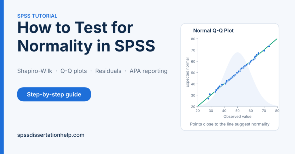
To test for normality in SPSS, go to Analyze → Descriptive Statistics → Explore, move your variable into the Dependent List, click Plots, tick Normality plots with tests, and click OK. SPSS returns a Tests of Normality table with the Shapiro-Wilk and Kolmogorov-Smirnov tests, plus a normal Q-Q plot. A Shapiro-Wilk p value above .05 means no significant departure from normality was detected; a value below .05 suggests the data depart from a normal distribution. That p value is only half the answer, though. You also need to test the right variable for your analysis, read the plots, and take sample size into account before deciding what to do.
This guide shows each step, explains what the output means, and gives you APA-ready wording for your dissertation.
In this guide
- What does normality mean?
- Why normality matters (and when it matters less)
- Which variable should you test?
- How to test for normality in SPSS, step by step
- How to interpret the Tests of Normality table
- How to read histograms and Q-Q plots
- Using skewness and kurtosis as a supporting check
- What to do if your data are not normal
- How to report normality in APA style
- Common mistakes
- When to get expert help
- Frequently asked questions
What Does “Normality” Mean in Statistics?
A normal distribution is the symmetrical, bell-shaped distribution in which most values cluster around the mean and fewer values appear the further you move into either tail. In a perfectly normal distribution, the mean, median and mode are equal, skewness is 0 and excess kurtosis is 0.
Real data are never perfectly normal. The practical question is whether the departure is large enough to affect your chosen test. That is why normality checking combines formal tests, plots and descriptive statistics rather than relying on a single number.
Why Normality Matters (and When It Matters Less)
Parametric tests such as the t test, ANOVA, Pearson correlation and linear regression assume that something in your data is approximately normal. When that assumption fails badly, p values and confidence intervals can be inaccurate, especially in small samples.
The assumption matters less as sample size grows. Because of the central limit theorem, the sampling distribution of the mean tends towards normality in larger samples even when the raw data are not normal. Ghasemi and Zahediasl (2012) note that with samples larger than about 30 or 40, violations of normality should not cause major problems for many parametric procedures. Treat this as a guideline, not a guarantee: strong skew, heavy tails or outliers can still distort results in moderate samples.
Which Variable Should You Test for Normality?
This is where most students go wrong. The normality assumption rarely applies to “all your variables”. It applies to a specific quantity, which depends on the analysis.
Table 1. Which Variable Should You Test for Normality?
| Analysis | What must be approximately normal | What to test in SPSS | Notes |
|---|---|---|---|
| Independent-samples t test | The outcome within each group | The dependent variable, with the group variable in the Factor List | Test each group separately |
| Paired-samples t test | The difference scores | A computed difference variable (post − pre) | Not the two time points separately |
| One-way ANOVA | The outcome within each group (equivalently, the residuals) | Dependent variable by group, or saved residuals | With many small groups, residuals are more informative |
| Pearson correlation | Each variable, and their joint pattern | Each variable, plus a scatterplot | Check for outliers and curved relationships |
| Linear regression | The residuals | Residuals saved from the regression | Predictors do not need to be normal |
| ANCOVA and factorial ANOVA | The residuals | Residuals saved from GLM Univariate | Testing raw groups ignores the covariate |
For the full list of assumptions behind each test, see our guides to the assumptions of the t test and testing the assumptions of linear regression.
Not sure which variable your supervisor expects you to test? Our SPSS dissertation help team can review your analysis plan and output with you, starting with a free initial consultation.
How to Test for Normality in SPSS (Step by Step)
The Explore procedure is the standard way to test for normality in SPSS because it produces the formal tests, plots and descriptive statistics in one run. Menu labels can differ slightly between SPSS versions; the syntax below works across versions.
Method 1: Explore With Normality Plots and Tests
- Go to Analyze → Descriptive Statistics → Explore.
- Move the variable you want to test into the Dependent List.
- If you are comparing groups (a t test or ANOVA), move the grouping variable into the Factor List. SPSS will then test each group separately.
- Optionally, move your participant ID into Label Cases by, so any unusual points on the plots are labelled with an ID rather than a row number.
- Click Plots. Tick Normality plots with tests and Histogram. Under Boxplots, choose Factor levels together. Click Continue.
- Under Display, choose Both, then click OK.
SPSS produces a Descriptives table (including skewness and kurtosis), a Tests of Normality table, a histogram, a normal Q-Q plot, a detrended normal Q-Q plot and a boxplot for each variable or group.
SPSS Syntax for Normality Testing
Saving syntax makes your analysis reproducible, which examiners increasingly expect.
EXAMINE VARIABLES=score BY group
  /ID=participant_id
  /PLOT BOXPLOT HISTOGRAM NPPLOT
  /COMPARE GROUPS
  /STATISTICS DESCRIPTIVES
  /CINTERVAL 95
  /MISSING LISTWISE
  /NOTOTAL.
Replace score, group and participant_id with your own variable names. NPPLOT is the keyword that produces the normality tests and Q-Q plots. If you have no grouping variable, remove BY group and /NOTOTAL.
Testing Residuals for Regression and ANOVA
For regression, ANCOVA and factorial ANOVA, save the residuals first and then test them with Explore.
Linear regression
- Go to Analyze → Regression → Linear and set up your model.
- Click Save. Under Residuals, tick Unstandardized (or Standardized). Click Continue, then OK.
- SPSS adds a new variable to your data file (for example
RES_1orZRE_1). - Run Explore on that residual variable, with no Factor List.
ANOVA, ANCOVA and factorial designs
- Go to Analyze → General Linear Model → Univariate and set up your model.
- Click Save, tick Unstandardized under Residuals, click Continue, then OK.
- Run Explore on the saved residual variable.
The Linear Regression dialog also offers a histogram and normal P-P plot of standardized residuals under Plots. These are useful visual checks alongside the saved-residual test.
Testing Difference Scores for a Paired t Test
- Go to Transform → Compute Variable.
- Name the target variable (for example
diff) and enter the expressionpost_score - pre_score. - Click OK, then run Explore on
diff.
COMPUTE diff = post_score - pre_score.
EXECUTE.
EXAMINE VARIABLES=diff
  /PLOT HISTOGRAM NPPLOT
  /STATISTICS DESCRIPTIVES.
How to Interpret the Tests of Normality Table in SPSS
The Tests of Normality table reports two tests side by side. Both test the same null hypothesis: that the data come from a normally distributed population.
Table 2. How to Read the SPSS Tests of Normality Table
| Column in output | What it means | What to look for | Common misreading |
|---|---|---|---|
| Kolmogorov-Smirnovᵃ Statistic | Largest distance between your data and a normal distribution, with the Lilliefors correction (footnote a) | Smaller is closer to normal | Confusing it with the one-sample K-S test under Nonparametric Tests, which is a different procedure |
| Shapiro-Wilk Statistic (W) | How closely the ordered data match the values expected under normality | Values close to 1 indicate closer agreement | Treating W = .95 as “95% normal” |
| df | The number of cases in that variable or group | Should match your sample or group size | Reading it as n − 1 |
| Sig. | The p value for the test | p < .05: a significant departure from normality was detected | Treating p > .05 as proof the data are normal |
| .200* in the K-S column | SPSS footnote: “This is a lower bound of the true significance” | Read as p ≥ .200 | Reporting it as exactly .200 |
How to decide. A non-significant result (p > .05) means the test found no evidence of a departure from normality. It does not prove that the data are normal, particularly in small samples where the test has little power. A significant result (p < .05) means a departure was detected, but in a large sample that departure may be too small to matter. Always look at the plots before deciding.
Shapiro-Wilk vs Kolmogorov-Smirnov: Which Should You Report?
Report Shapiro-Wilk as your main test in most dissertation designs. Simulation studies have found that it detects departures from normality more reliably than the Kolmogorov-Smirnov and Lilliefors tests (Razali & Wah, 2011; Ghasemi & Zahediasl, 2012). If the two tests disagree, base your decision on Shapiro-Wilk together with the plots, and say so in your write-up.
Why Sample Size Changes What the p Value Means
Normality tests are hypothesis tests, so their results depend heavily on sample size.
- Small samples (for example, n < 30): the tests have low power and often return p > .05 even when the data are clearly skewed. Plots and skewness/kurtosis matter more here.
- Large samples (several hundred cases): the tests become so sensitive that trivial, harmless departures produce p < .05. At the same time, the central limit theorem makes tests on means more robust.
This is why a significant Shapiro-Wilk result in a sample of 500 does not automatically mean you should abandon a t test or ANOVA, and why a non-significant result in a sample of 15 is not reassuring on its own.
How to Read Histograms and Q-Q Plots in SPSS
The normal Q-Q plot compares each observed value with the value expected if the data were normal. If the data are normal, the points fall close to the straight diagonal line.
- Points close to the line along its full length: approximately normal.
- A curved, banana-shaped pattern: skewness. The direction of the bend shows which tail is longer; compare it with the histogram to confirm.
- An S-shape, with both ends pulling away in opposite directions: heavy or light tails (kurtosis).
- One or two points far from the line at an end: possible outliers. Check them before drawing conclusions; see our guide on how to check for outliers in SPSS.
The detrended normal Q-Q plot shows each point’s vertical distance from the line. Points scattered randomly around zero indicate normality; a clear curve or U-shape indicates a systematic departure.
The histogram gives an overall impression of shape, but its appearance changes with the number of bars, so use it alongside the Q-Q plot rather than on its own.
Using Skewness and Kurtosis as a Supporting Check
The Descriptives table from Explore reports skewness and kurtosis with their standard errors. Dividing each statistic by its standard error gives a z value. Kim (2013) suggests sample-size-dependent cut-offs:
- n < 50: an absolute z above 1.96 suggests non-normality.
- n between 50 and 300: an absolute z above 3.29 suggests non-normality.
- n above 300: ignore the z values and look at the absolute statistics; skewness beyond ±2 or kurtosis beyond 7 (on the “proper” kurtosis scale, roughly 4 on the excess-kurtosis scale SPSS reports) indicates substantial non-normality.
These are conventions, and other textbooks use slightly different values. For a fuller explanation of what skewness and kurtosis show, see how to interpret skewness and kurtosis.
What to Do If Your Data Are Not Normally Distributed
A significant normality test is a reason to look closer, not a reason to panic. Work through these options in order.
Table 3. What to Do If Your Data Are Not Normal
| Situation | Likely cause | Recommended option | What to report |
|---|---|---|---|
| One or two extreme points drive the result | Data-entry error or outlier | Check the source data; correct errors; investigate genuine outliers before removing anything | What was found and what was done |
| Large sample, plots look close to normal, test is significant | Test oversensitivity | Proceed with the parametric test; justify with the plots and sample size | Test result, plots and the justification |
| Clear positive skew (e.g., income, reaction times, counts) | Naturally skewed variable | Consider a log or square-root transformation, or a nonparametric test | The transformation and that results refer to transformed data |
| Small sample with clear non-normality | Low robustness | Use the nonparametric alternative (Table 4) | Why the nonparametric test was chosen |
| Non-normal residuals in regression | Misspecified model, outliers or skewed outcome | Check for curvature and outliers; consider transformation or bootstrapped confidence intervals | Diagnostics and the remedy used |
| Ordinal data (single Likert items) | Normality not meaningful | Use a nonparametric test | The measurement-level rationale |
Table 4. Parametric Tests and Their Nonparametric Alternatives
| Parametric test | Nonparametric alternative |
|---|---|
| Independent-samples t test | Mann-Whitney U test |
| Paired-samples t test | Wilcoxon signed-rank test |
| One-way ANOVA | Kruskal-Wallis test |
| Pearson correlation | Spearman’s rank-order correlation |
Transformation steps are covered in how to transform variables in SPSS, and the wider choice between test families in parametric and non-parametric tests. Remember that transforming changes how you interpret the results, and nonparametric tests answer a slightly different question (usually about ranks or medians rather than means).
Not sure whether to transform, switch tests or proceed? Send us your SPSS output and research questions, and a statistician will recommend the most defensible option for your design. Request a free initial review.
How to Report Normality Tests in APA Style
State which test you used, the statistic with its degrees of freedom, the p value, what the plots showed, and the decision you took. The examples below are illustrative: the numbers are invented to show the wording.
Example 1: Normality supported
The assumption of normality was assessed using the Shapiro-Wilk test and inspection of normal Q-Q plots. Exam scores were approximately normally distributed in both the intervention group, W(42) = .97, p = .34, and the control group, W(40) = .96, p = .19, and the Q-Q plots showed no marked departures from the diagonal.
Example 2: Significant test, parametric analysis retained
The Shapiro-Wilk test indicated a departure from normality for the regression residuals, W(312) = .99, p = .02. However, the normal Q-Q plot showed only minor deviation in the tails, skewness (0.21) and kurtosis (0.38) were close to zero, and the sample was large. Given the robustness of regression to small departures in samples of this size, the analysis proceeded as planned.
Example 3: Non-normal data, nonparametric test used
Anxiety scores were positively skewed in both groups (Shapiro-Wilk, W(18) = .84, p = .006, and W(17) = .86, p = .014), and the Q-Q plots confirmed the departure. Given the small group sizes, a Mann-Whitney U test was used instead of an independent-samples t test.
For broader formatting rules, see how to report SPSS results in APA format.
Common Mistakes When Testing Normality in SPSS
- Testing the wrong variable. Testing raw predictors for regression, or each time point for a paired t test, instead of the residuals or difference scores.
- Testing the whole sample when comparing groups. Use the Factor List so each group is tested separately.
- Treating p > .05 as proof of normality. It only means no departure was detected.
- Abandoning a parametric test because of a significant result in a large sample. Check the plots and the size of the departure first.
- Relying on the p value alone. Always inspect the Q-Q plot.
- Reporting Kolmogorov-Smirnov only. Shapiro-Wilk is generally the more powerful test.
- Reporting “.200” as an exact p value. The asterisk means it is a lower bound.
- Testing single Likert items for normality. Ordinal items with five or seven options are not continuous; test composite scale scores instead, or use nonparametric methods.
- Deleting cases until the test turns non-significant. This biases your results and must never be done.
When to Get Expert Help
Normality checking is quick to run but easy to misjudge. Consider getting help if:
- Shapiro-Wilk and the Q-Q plot point in different directions
- Your large sample fails every normality test
- You are unsure whether to test raw variables or residuals
- Your supervisor has questioned your assumption checks
- You need to decide between transforming, switching tests or bootstrapping
- Your deadline does not leave time to rerun the analysis
Our SPSS statisticians check assumptions, choose the appropriate test for your design, run the analysis, and deliver annotated output, reusable syntax and APA 7 tables, with support for your results chapter if you need it. Pricing is quote-based: it depends on your academic level, discipline, deadline and writer category, with turnaround options from a few hours to two weeks. Everything is confidential, and you keep control of your research decisions.
Request a quote · See how pricing works
Frequently Asked Questions
Shapiro-Wilk is generally recommended because simulation studies show it detects departures from normality more reliably than Kolmogorov-Smirnov. Use it together with a normal Q-Q plot rather than on its own.
Explore reports both the Kolmogorov-Smirnov test (with the Lilliefors correction) and the Shapiro-Wilk test. They use different methods and can occasionally disagree; most researchers report Shapiro-Wilk.
A p value below .05 means the test detected a statistically significant departure from a normal distribution. Whether that departure matters depends on its size, your sample size and your analysis.
Not necessarily. A non-significant result means no departure was detected. In small samples the test may simply lack the power to detect one, so check the Q-Q plot and skewness as well.
Yes, but on the residuals, not the raw variables. Save the residuals from the regression and test them with Explore. Predictors do not need to be normally distributed.
Often yes, if the sample is moderately large and the departure is not severe, because the t test is fairly robust. In small samples with clear skew, a Mann-Whitney U test (independent groups) or Wilcoxon signed-rank test (paired data) is usually safer.
Report the statistic, degrees of freedom and p value, for example W(40) = .96, p = .19, together with a sentence on what the Q-Q plots showed and the decision you made.
Final Thoughts
Testing for normality in SPSS takes a few clicks; interpreting it well takes judgement. Test the right variable for your analysis, read the Shapiro-Wilk result together with the Q-Q plot, weigh your sample size, and report what you found and why you chose your next step. That combination is what examiners look for in a methods and results chapter.