Mauchly’s test of sphericity checks whether the variances of the differences between every pair of levels in a repeated measures factor are equal. SPSS displays it automatically whenever a within-subjects factor has three or more levels. If the test is significant (Sig. < .05), don’t report the uncorrected ANOVA row; read the Greenhouse-Geisser or Huynh-Feldt corrected row instead.
When Sphericity Matters
Sphericity is an assumption underneath repeated measures ANOVA, not a separate test you run on your raw data. It’s worth distinguishing it from two assumptions it’s often confused with:
- Sphericity concerns the variances of the difference scores between each pair of repeated conditions. If you measure the same participants at three time points, sphericity asks whether Var(Time1 minus Time2), Var(Time1 minus Time3), and Var(Time2 minus Time3) are all roughly equal.
- Homogeneity of variance (checked with Levene’s test) concerns whether groups have equal variance on the raw dependent variable, and applies to between-subjects comparisons.
- Bartlett’s test of sphericity, which appears in factor analysis, checks something else entirely: whether a correlation matrix is an identity matrix, which tells you whether factor analysis is appropriate for the data at all. It is unrelated to the repeated measures assumption despite the similar name.
Sphericity only becomes a live question when a within-subjects factor has three or more levels. With exactly two levels there is only one pairwise difference to compute, so there is nothing for its variance to differ from: the assumption is met by construction, and SPSS does not print a Mauchly’s Test table for that effect.
Example: A researcher measures the same 30 participants’ anxiety scores before treatment, immediately after treatment, and at a one-month follow-up. Because there are three repeated levels, Mauchly’s test is relevant and SPSS will report it automatically when the repeated measures ANOVA is run.
Step-by-Step: Finding Mauchly’s Test in SPSS
Mauchly’s test is not a procedure you request separately. It is produced as a byproduct of running a repeated measures ANOVA.
- Go to Analyze > General Linear Model > Repeated Measures…
- In the Repeated Measures Define Factor(s) dialog, name your within-subjects factor and enter the Number of Levels (3 or more, for the test to be relevant), then click Add and Define.
- Move your repeated measurement variables into the Within-Subjects Variables box in the order that matches the levels you defined.
- Click OK to run the procedure. No separate checkbox is needed: IBM’s documentation confirms that Mauchly’s test is displayed automatically for a repeated measures analysis.
- In the Viewer, locate the table titled Mauchly’s Test of Sphericityᵇ. It appears before the Tests of Within-Subjects Effects table.
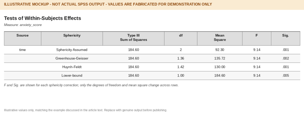
- Read the Tests of Within-Subjects Effects table directly below it. This table lists four rows for your within-subjects effect: Sphericity Assumed, Greenhouse-Geisser, Huynh-Feldt, and Lower-bound, each with its own degrees of freedom and F test based on the same underlying data.
This process is an assumption check inside your repeated measures ANOVA, not a separate analysis that replaces it. You still need the ANOVA to answer your research question; Mauchly’s test only tells you which row of that ANOVA’s output to trust.
Walking Through an Illustrative Output Example
All numbers below are illustrative, not from a real dataset or study.
Suppose a repeated measures ANOVA on the three-timepoint anxiety example above produces this Mauchly’s test row:
Mauchly’s W = .81, Approx. Chi-Square = 5.92, df = 2, Sig. = .052 Epsilon: Greenhouse-Geisser = .84, Huynh-Feldt = .89, Lower-bound = .50
Here Sig. is just above the conventional .05 threshold, so on a strict reading sphericity is not rejected. Because the result sits close to the threshold, a careful write-up would still mention the epsilon values and note that sphericity was only marginally tenable, rather than treating .052 as unambiguous confirmation.
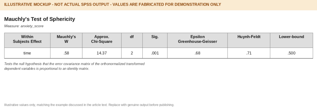
Now suppose a second, separate illustrative example produces:
Mauchly’s W = .58, Approx. Chi-Square = 14.37, df = 2, Sig. = .001 Epsilon: Greenhouse-Geisser = .68, Huynh-Feldt = .71, Lower-bound = .50
Here Sig. is well below .05, so sphericity is violated. The Tests of Within-Subjects Effects table for this example might show:
Sphericity Assumed: F(2, 58) = 9.14, p = .001 Greenhouse-Geisser: F(1.36, 39.44) = 9.14, p = .002
Notice the F value doesn’t change between corrections; only the degrees of freedom shrink, which changes the p value the F is evaluated against.
Decision Table: What to Report
| Mauchly’s test result | What to inspect | What to report |
|---|---|---|
| Sig. ≥ .05 (not significant) | Confirm the within-subjects factor has 3+ levels and the result isn’t borderline | The Sphericity Assumed row of the Tests of Within-Subjects Effects table |
| Sig. < .05 (significant) | The epsilon estimates (Greenhouse-Geisser, Huynh-Feldt) | A corrected row: Greenhouse-Geisser or Huynh-Feldt, per your analysis plan |
| No Mauchly’s table appears | Whether the within-subjects factor has exactly 2 levels | The Sphericity Assumed row; correction is not applicable with 2 levels |
On choosing between Greenhouse-Geisser and Huynh-Feldt: some textbooks describe a rule of thumb based on the size of epsilon, but treating any single cutoff as a universal rule oversimplifies the decision. Which correction to prefer, and how conservatively to interpret a borderline Mauchly’s result, should follow your study’s preregistered analysis plan or your field’s methodological guidance, not a single number applied automatically. When in doubt, consult a statistics reference appropriate to your discipline or your dissertation committee’s preferred convention.
How to Report It in APA Style
Both examples are illustrative and should be replaced with your own output.
Sphericity assumed (illustrative):
Mauchly’s test indicated that the assumption of sphericity had not been violated, χ²(2) = 5.92, p = .052. A repeated measures ANOVA showed a significant effect of time on anxiety scores, F(2, 58) = 9.14, p = .001.
Sphericity violated, correction applied (illustrative):
Mauchly’s test indicated that the assumption of sphericity had been violated, χ²(2) = 14.37, p = .001. Therefore, degrees of freedom were corrected using Greenhouse-Geisser estimates of sphericity (ε = .68). The effect of time on anxiety scores remained significant, F(1.36, 39.44) = 9.14, p = .002.
Common Mistakes to Avoid
- Treating a nonsignificant result as proof of sphericity. A Sig. of .052 or .20 means the test did not detect a violation; it does not confirm the assumption holds, particularly in small samples where the test has limited power.
- Reporting the uncorrected ANOVA after a significant Mauchly’s test, without explanation. If sphericity is violated and you still report Sphericity Assumed, say why (for example, that the F-test is robust to the specific violation observed, with a cited justification), rather than silently ignoring the correction.
- Confusing Mauchly’s test with the ANOVA result itself. Mauchly’s Sig. value tells you which row of the ANOVA table to trust; it is not itself a test of your research hypothesis about condition means.
- Requesting or expecting Mauchly’s test for a two-level within-subjects factor. SPSS omits the table in this case because the assumption is trivially satisfied, not because of an error in the analysis.
Frequently Asked Questions
This almost always means the factor has exactly two levels. With only one pairwise difference to evaluate, sphericity cannot be violated, so SPSS doesn’t print the test.
Greenhouse-Geisser generally produces a more conservative (smaller) epsilon than Huynh-Feldt, particularly when epsilon is far below 1, which is one reason some analysts default to it when uncertain. This is a general tendency, not a fixed rule for every dataset.
Not really; in SPSS’s GLM Repeated Measures procedure, it is produced alongside the ANOVA as a diagnostic, not as a standalone command you can request in isolation.
This can happen and is one reason to look at the epsilon values themselves rather than only the Sig. column; a statistically significant departure from perfect sphericity does not necessarily correspond to a practically large one, especially with large sample sizes.
Next Steps
Mauchly’s test settles one specific question: which row of your repeated measures ANOVA output to trust. It doesn’t replace the substantive interpretation of your F-test, your effect sizes, or your study’s broader analysis plan. For help running and interpreting the full repeated measures ANOVA, including between-subjects factors, post hoc comparisons, and effect sizes, see our Repeated Measures ANOVA SPSS Help page.